ae-06-solution

Read in Data

# A tibble: 6 × 9
    Age Gender   BMI BPSysAve BPDiaAve DirectChol TotChol Diabetes PhysActive
  <int> <fct>  <dbl>    <int>    <int>      <dbl>   <dbl> <fct>    <fct>     
1    34 male    32.2      113       85       1.29    3.49 No       No        
2    49 female  30.6      112       75       1.16    6.7  No       No        
3    45 female  27.2      118       64       2.12    5.82 No       Yes       
4    58 male    23.7      104       74       0.96    4.24 No       Yes       
5    54 male    26.0      134       85       1.16    6.41 No       Yes       
6    58 female  26.2      127       83       1.14    4.78 No       Yes

Exercise 1

(a)

cor_pearson <- cor(nhanes_clean$BPSysAve, 
                   nhanes_clean$Age, 
                   method = "pearson")
cor_pearson

[1] 0.3208457

Interpretation: The Pearson correlation coefficient is 0.321, indicating a moderate positive linear relationship between systolic blood pressure and age. As age increases, systolic blood pressure tends to increase.

(b)

cor_spearman <- cor(nhanes_clean$BPSysAve, 
                    nhanes_clean$Age, 
                    method = "spearman")

Interpretation: The Spearman correlation coefficient is 0.32, which is similar to the Pearson correlation. Spearman correlation measures monotonic (not necessarily linear) relationships and is based on ranks rather than raw values. It is preferred when: (1) the relationship is monotonic but not linear or (2) data contain outliers that would affect Pearson. In this case, both correlations are similar, suggesting the relationship is approximately linear.

(c)

ggplot(nhanes_clean, aes(x = Age, y = BPSysAve)) +
  geom_point(alpha = 0.3, size = 1) +
  geom_smooth(method = "lm", color = "blue", se = TRUE) +
  labs(title = "Relationship between Age and Systolic Blood Pressure",
       x = "Age (years)",
       y = "Systolic Blood Pressure (mmHg)") +
  theme_minimal()

`geom_smooth()` using formula = 'y ~ x'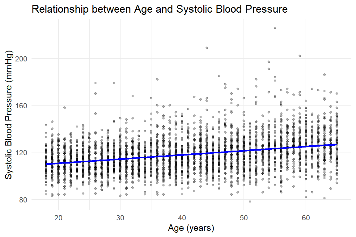

Slight positive trend, matches the correlations from (a) and (b).

Exercise 2

(a)

\[\text{BPSysAve}_i = \beta_0 + \beta_1 \times \text{Age}_i + \epsilon_i, \quad i = 1, \ldots, n\]

\(\text{BPSysAve}_i\) = systolic blood pressure for person \(i\)
\(\beta_0\) = intercept (expected BP when age = 0)
\(\beta_1\) = slope (change in BP per 1-year increase in age)
\(\text{Age}_i\) = age for person \(i\)
\(\epsilon_i\) = residual error for person \(i\), assumed \(\epsilon_i \sim N(0, \sigma^2)\) independently

(b)

The error is unobserved (unknown population parameter), the residual is observed and is defined as \(y_i - \hat y_i\).

(c)

model1 <- lm(BPSysAve ~ Age, data = nhanes_clean)
tidy(model1) |>
  kable(digits = 3)

term	estimate	std.error	statistic	p.value
(Intercept)	103.596	0.749	138.390	0
Age	0.356	0.018	20.325	0

(d)

Interpretation: The slope coefficient for Age is 0.356, meaning that for each additional year of age, systolic blood pressure increases by approximately 0.356 mmHg, on average.

The p-value tests: - \(H_0: \beta_1 = 0\) (no linear relationship between age and BP) - \(H_A: \beta_1 \neq 0\) (there is a linear relationship)

The p-value is < 0.001, so we reject the null hypothesis and conclude there is strong evidence of a linear relationship between age and systolic blood pressure. The test statistic follows a t-distribution with \(n-2 = 3600\) degrees of freedom.

Exercise 3

(a)

model1_diag <- augment(model1)

# 1. Residuals vs Fitted (Linearity)
p1 <- ggplot(model1_diag, aes(x = .fitted, y = .resid)) +
  geom_point(alpha = 0.3) +
  geom_hline(yintercept = 0, color = "red", linetype = "dashed") +
  geom_smooth(se = FALSE, color = "blue") +
  labs(title = "Residuals vs Fitted",
       x = "Fitted values",
       y = "Residuals") +
  theme_minimal()

# 2. Q-Q Plot (Normality)
p2 <- ggplot(model1_diag, aes(sample = .resid)) +
  stat_qq() +
  stat_qq_line(color = "red") +
  labs(title = "Normal Q-Q Plot",
       x = "Theoretical Quantiles",
       y = "Sample Quantiles") +
  theme_minimal()

# 3. Homoscedasticity
p3 <- ggplot(model1_diag, aes(x = .resid)) +
  geom_histogram(alpha = 0.3) +
  labs(x = "Residuals") +
  theme_minimal()

(p1 | p2) / (p3)

`geom_smooth()` using method = 'gam' and formula = 'y ~ s(x, bs = "cs")'
`stat_bin()` using `bins = 30`. Pick better value `binwidth`.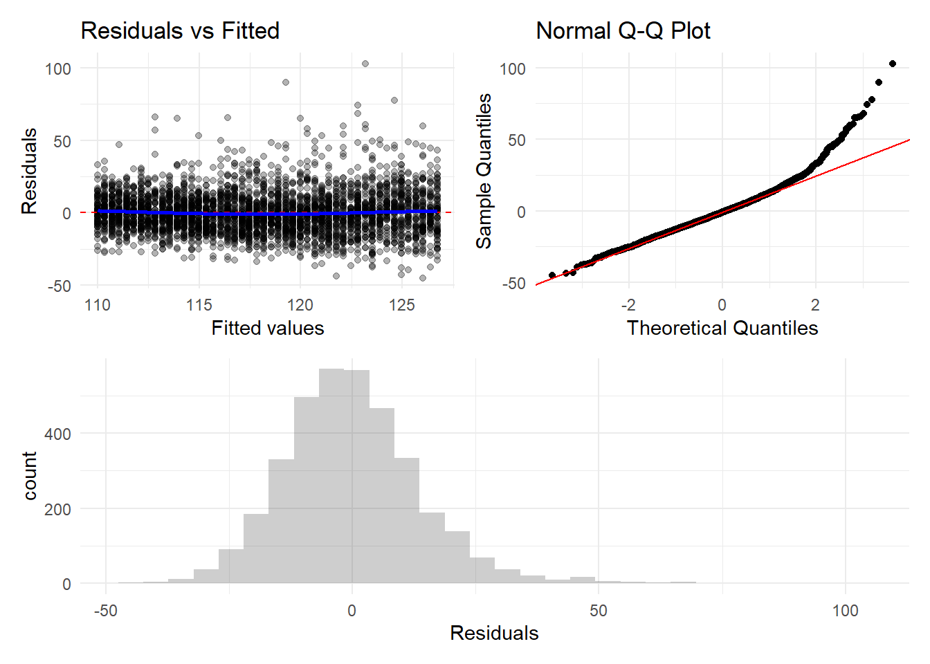

(b)

Linearity: The Residuals vs Fitted plot shows a relatively random scatter around zero with no clear pattern, suggesting the linearity assumption is reasonably met. The relationship between age and BP appears to be approximately linear.
Normality: The Q-Q plot shows that residuals mostly follow the diagonal line, with slight deviations in the tails. The histogram shows an approximately normal distribution with slight right skew. Overall, the normality assumption is reasonably satisfied for inference purposes.
Homoscedasticity (constant variance): The fitted vs. residuals plot shows a relatively horizontal line with roughly equal spread of residuals across fitted values. There might be slightly more variance at higher fitted values, but the assumption appears adequately met.
Independence: We cannot fully assess independence from these plots alone. However, there’s no obvious pattern in the Residuals vs Fitted plot suggesting dependence. Since each observation is a different person and we’ve removed duplicates, independence is likely satisfied. If observations were collected over time or in clusters, we’d need to investigate further.

Exercise 4

(a)

model2 <- lm(BPSysAve ~ Age + BMI + Gender, 
             data = nhanes_clean)
tidy(model2) |>
  kable(digits = 3)

term	estimate	std.error	statistic
(Intercept)	90.456	1.147	78.866
Age	0.331	0.017	19.636
BMI	0.374	0.033	11.465
Gendermale	6.644	0.455	14.592

(b)

BMI (0.374): For each 1-unit increase in BMI, systolic BP increases by 0.374 mmHg, holding age and gender constant.

(c)

rsq <- summary(model2)$r.squared
adj_rsq <- summary(model2)$adj.r.squared

cat("R-squared:", round(rsq, 4), "\n")

R-squared: 0.1791

cat("Adjusted R-squared:", round(adj_rsq, 4), "\n")

Adjusted R-squared: 0.1784

17.9% of the variation in systolic blood pressure is explained by age, BMI, and gender in our model.

The adjusted \(R^2\) adjusts for the number of predictors in the model, penalizing for adding variables that don’t improve the model. It’s useful for comparing models with different numbers of predictors.

(d)

Interpretation: The global F-test tests:

\(H_0\): All coefficients except the intercept are zero (\(\beta_1 = \beta_2 = \beta_3 = 0\))
\(H_A\): At least one coefficient is non-zero (at least one nonzero linear association between a predictor and the outcome.)

The F-statistic follows an F-distribution with 3 and 3602- 4 = 3598 degrees of freedom (df1 = number of predictors = 3, df2 = n - number of parameters = n - 4).

The p-value is < 0.001, so we reject the null hypothesis and conclude that our model with age, BMI, and gender provides significantly better predictions than a model with only an intercept. At least one predictor is significantly related to systolic BP.

(e)

\(\hat \text{SBP} = 90.456 + 0.331(45) + .374(28) + 6.664(1)\)

90.456+0.331*45 + 3.74*28 + 6.664

[1] 216.735

We’d expect the blood pressure to be 216.735 mmHg.

Exercise 5

# Use the CO2 dataset (plant CO2 uptake experiment)
data(CO2)

# Create binary outcome: High CO2 uptake (above median)
co2_data <- CO2 |>
  mutate(high_uptake = ifelse(uptake > median(uptake), 1, 0))

# Fit logistic regression
# Predicting high CO2 uptake from concentration, temperature, and treatment
model_co2 <- glm(high_uptake ~ conc + 
                   Treatment + 
                   Type, 
                 data = co2_data, 
                 family = binomial)
tidy(model_co2) |>
  kable(digits = 3)

term	estimate	std.error	statistic	p.value
(Intercept)	0.834	0.697	1.198	0.231
conc	0.005	0.001	3.640	0.000
Treatmentchilled	-2.355	0.750	-3.139	0.002
TypeMississippi	-3.770	0.849	-4.439	0.000

(a)

For plants with chilled treatment, the odds of high C02 uptake are multiplied by a factor of exp(-2.355) compared to those with nonchilled treatment, holding plant origin and concentration constant.

Equivalent: Plants with chilled treatment is associated with a 91% lower odds of high C02 uptake rate compared to plants w/ non-chilled treatment, holding other predictors constant.

(b)

Each one ml/L increase in ambient C02 concentration is associated with the odds of high C02 uptake being multiplied by exp(.005), holding origin and treatment constant.

Equivalent: A one ml/L increase in ambient C02 concentration is associated with a .5% increase in odds of high C02 uptake rate, holding origin and treatment type constant.