my_data <- data.frame(
  id = 1:5,name = c("Alice", 'Bob', "Charlie", "David", "Eve"),
  score=c(85,92,78,95,88)
)In-Class Review Questions
Exam 02 Preparation
- How can the below code be improved according to good coding style?
- How can the below code be improved according to good coding style?
df <- data.frame(grp = c("A","A","B","B","C","C"),
val=c(10,15,20,25,30,28))

ggplot(df, aes(x = grp,y=val)) +
  geom_boxplot()+geom_point(position = position_jitter(width = .1))

meanvaluefromdataframe <- df |>
group_by(grp) |> summarise(m = mean(val))- How can the below code be improved according to good coding style?
ggplot(mtcars, aes(wt, mpg, colour=factor(      cyl), shape = factor(vs))) +
       geom_point() +theme(legend.text = element_text(size = 8, colour = 'red'))
Suppose you have 100 samples of 100 observations each that are binary (0/1), each with probability of success \(p=.3\). What does the Central Limit Theorem say about the distribution of sample averages? (In other words, what would a histogram of the sample averages look like? Centered around which value?) What if our observations were drawn from a continuous but skewed population distribution?
Researchers compare fasting glucose levels measured before and after a 12-week exercise program among the same participants.
Which type of t-test should they use & why?
Write the null hypothesis in words. What would the alternative for a two-sided test be? How about for a one-sided test?
A new rapid test for strep throat is being evaluated. Assume that \(H_0\) is that the person truly doesn’t have strep throat. What would a Type I error mean? What would a Type II error mean? What is a danger of a Type I error here? What is a danger of a Type II error here?
Explain how the t-distribution differs from the standard normal distribution. When would we use a t-distribution instead of Z?
Write the R code to find the following (on exams, you won’t need to write code):
The 95th percentile of a t(df = 12) distribution.
The probability that a
t(df = 8)random variable is greater than 2.1.The 90th percentile of a \(N(\mu = 3, \sigma = 5)\) distribution.
What is the definition of a p-value?
Researchers are studying whether a new herbal supplement helps reduce recovery time after a mild viral infection compared to a placebo. Ten participants were randomly assigned to either the supplement group or the placebo group. After recovery, the number of days until full recovery was recorded:
| Group | Recovery Time (days) |
|---|---|
| Supplement | 4, 6, 5, 7, 6 |
| Placebo | 8, 9, 6, 10, 9 |
Because the data are not normally distributed, the researchers decide to use a Mann–Whitney U test.
State the null and alternative hypotheses for a two-sided test in words.
Using R, we can calculate the test statistic with
wilcox.test. See output below (note you will not be expected to know this function for the exam, but you should know how to interpret p-value for these tests):
# Data
supplement <- c(4, 6, 5, 7, 6)
placebo <- c(8, 9, 6, 10, 9)

# Mann–Whitney U test
wilcox.test(supplement, placebo, alternative = "two.sided")
    Wilcoxon rank sum test with continuity correction

data:  supplement and placebo
W = 2, p-value = 0.03389
alternative hypothesis: true location shift is not equal to 0
What is your conclusion, using \(\alpha = .05\)?
- Suppose that instead we calculated a one-sided test. The new alternative would be the following:
\(H_A\): The supplement group has shorter recovery times than the placebo group.
Suppose that we computed the test-statistic and got a p-value of .25. What is your conclusion at a 5% significance level?
- Below are two power calculations. In which object (
p1orp2) will the power be higher? Why?
p1 <- power.t.test(n = 28,
             delta = 1.5,
             sd = 2.3,
             sig.level = 0.05,
             type = "two.sample",
             alternative = "two.sided")

p2 <- power.t.test(n = 28,
             delta = 1.5,
             sd = 5,
             sig.level = 0.05,
             type = "two.sample",
             alternative = "two.sided")
Explain two reasons why it’s important to perform a power / sample size calculation during the design process of a study.
Dr. Stats is studying whether average daily sugar intake differs between two groups of teenagers: those who regularly eat breakfast and those who skip breakfast. She loads her dataset and runs the following code in R:
t.test(sugar ~ breakfast_group, data = teen_nutrition)What is this code doing? Describe in 1–2 sentences what is being compared and the test is being performed.
Specify the null and alternative hypothesis for this test in words and in symbols.
Suppose Dr. Stats looks at histograms of sugar intake for each group and sees that the distributions are heavily skewed with strong outliers. She wants a test that does not assume normality. What non‑parametric test corresponds to the two‑sample t‑test in this situation?
- Research shows that frequent involuntary police stops are associated with chronic stress and elevated cortisol levels. The average cortisol level in US adults is μ = 15 μg/dL, with a known population standard deviation of \(\sigma\) = 6 μg/dL. A public health researcher samples n = 50 adults from a neighborhood with documented high rates of police stops. The sample mean cortisol level is \(\bar{X}\) = 22.8 μg/dL.
Using the central limit theorem, write the formula for the test statistic \(Z = \frac{\bar{X} - \mu}{SE}\) where \(SE=\frac{\sigma}{\sqrt{n}}\) and substitute the given values into the expression. Leave as a fraction.
If the computed z‑statistic is very large in magnitude (far from 0), what would this tell the researcher about cortisol levels in this community?
State the null and alternative hypotheses in words and symbols for testing whether mean cortisol levels in this neighborhood differ from the national average
If the population standard deviation \(\sigma\) was unknown, what test would the researcher use instead of a z‑test?
Based on the output below, what conclusion should the researcher draw at \(\alpha\) = .05?
    One Sample t-test

data:  cortisol
t = 8.5764, df = 49, p-value = 2.545e-11
alternative hypothesis: true mean is not equal to 15
95 percent confidence interval:
 18.62547 20.84438
sample estimates:
mean of x
 19.73493
What is the distribution of our test statistical under the null hypothesis (include the name and the degrees of freedom, if applicable)
Interpret the 95% confidence interval in the context of the study.
Would the confidence interval be wider or smaller if you generated a 99% confidence interval?
- A researcher designing a two‑sample t‑test increases the sample size from n = 25 per group to n = 60 per group. How does this affect statistical power?
- Researchers are investigating whether residential proximity to a toxic waste site is associated with kidney function, measured by estimated glomerular filtration rate (eGFR, mL/min/1.73m²). Lower eGFR values indicate reduced kidney function. Adults were sampled from three distance zones from the nearest registered toxic waste site: less than 1 mile, 1–3 miles, and more than 3 miles away.
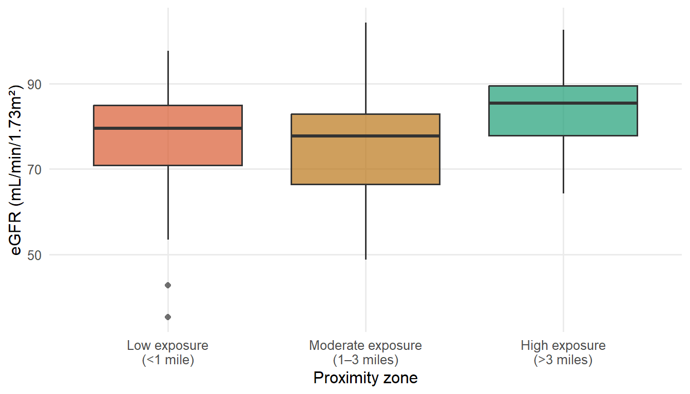
Write the null and alternative hypotheses for this ANOVA in words.
What does the F-statistic tell you about between-group variation in this study? What does a small F-statistic close to 1 suggest?
fit <- aov(egfr ~ zone, data = egfr_data)
summary(fit)
Df Sum Sq Mean Sq F value Pr(>F)
zone 2 1469 734.7 4.723 0.0113 *
Residuals 87 13535 155.6
---
Signif. codes: 0 '***' 0.001 '**' 0.01 '*' 0.05 '.' 0.1 ' ' 1Look at the ANOVA table above. Based on the ANOVA output, do you reject or fail to reject the null hypothesis at \(\alpha = .05\)? Justify your answer using the p-value from the table.
A classmate says: “The ANOVA was significant, but I still want to run pairwise t-tests between all three zone pairs to see which ones differ.” Should you run pairwise comparisons here? Explain in 1-2 sentences why or why not.
When you run the pairwise comparisons, there are three possible pairs. In 1–2 sentences, describe how you would adjust the significance rule to control the family-wise Type I error rate
- How does
st_readdiffer fromread.csv?
True/False
(True / False): The value returned by
qnorm(.95, mean = 0, sd = 1)is larger than the value returned byqnorm(.90, mean = 0, sd = 1)(True / False): Power is the probability of rejecting the null hypothesis when the null hypothesis is actually false.
(True / False): One assumption of an ANOVA is homoscedastic variance, i.e. that the within-group variance is the same for all groups.
(True / False): A p-value is the probability that the null hypothesis is true.
(True/False): A Type I error occurs when we fail to reject the null hypothesis even though the alternative hypothesis is actually true
(True / False): If we are using a significance level of \(\alpha=0.05\) and our p‑value is 0.20, we would accept the null hypothesis
The value returned by
pnorm(.3, mean = 0, sd = 1)is larger than the value returned bypnorm(.1, mean = 0, sd = 1)In a paired t-test, the two groups must be independent of each other.
Holding all else constant, decreasing alpha generally increases power.
A Fisher’s exact test is preferred over a chi-square test when sample counts in each cell are \(\geq 10\).
Holding all else constant, a confidence interval using \(\alpha = 0.05\) would be narrower compared to a confidence interval using \(\alpha = 0.01\).
(True / False): For three tests, to preserve an overall 0.05 Type I error rate, the Bonferroni correction would use \(\alpha/6 = .00083\) as the significance level for each individual test.