Call:
lm(formula = asthma ~ ., data = df)

Residuals:
   Min     1Q Median     3Q    Max
-4.968 -1.182  0.130  1.263  5.017

Coefficients:
            Estimate Std. Error t value Pr(>|t|)
(Intercept)  7.36391    1.13345   6.497 3.64e-09 ***
Pollutant1  -0.11830    0.17150  -0.690    0.492
Pollutant2   0.08736    0.16647   0.525    0.601
Pollutant3   0.10828    0.15910   0.681    0.498
---
Signif. codes:  0 '***' 0.001 '**' 0.01 '*' 0.05 '.' 0.1 ' ' 1

Residual standard error: 1.971 on 96 degrees of freedom
Multiple R-squared:  0.1202,    Adjusted R-squared:  0.09269
F-statistic: 4.371 on 3 and 96 DF, p-value: 0.006261Practice Problems
Some of these problems are meant to be fairly difficult–the purpose is to get you to think carefully about the concepts we’ve covered in class, and give you a better understanding of those underlying concepts, in order to be better prepared for the final.
Since some of these are a bit challenging, you are encouraged to discuss these problems in small groups.
Exercise 1: Multicollinearity and linear regression
A (fictional) study examined the association between three air pollutants, Pollutant1, Pollutant2, and Pollutant3, and prevalence of asthma within counties in a fictional U.S. state. The pollutant variables are the average concentrations in parts per billion (ppb) measured at monitoring sites within that county. Prevalence of asthma is the % of the county’s population diagnosed with asthma; it’s treated as normally distributed. The sample comprised 100 counties in this state. Assume hypothesis tests are conducted with significance level \(\alpha=.05.\)
(a)
Write out the model that has been fit in symbols below (i.e. \(Asthma_{i} = ...\))
(b)
What are the results of the hypothesis tests for the significance of each pollutant? Interpret these results in the context of the study.
(c)
Write the null and alternative hypotheses for the F-test for overall model significance. Write these hypotheses both in symbols, and in words in the context of the study.
(d)
What is the result of the overall F-test for the linear regression model? Interpret this result in the context of the study.
(e)
Do these results show indication of possible multicollinearity affecting this model? Why or why not?
(f)
The researchers decide to check for multicollinearity as follows:
library(car)
vif(fit)
Pollutant1 Pollutant2 Pollutant3
62.52846 57.92934 53.92988 What did the researchers do? Explain in 1 sentence. What do the results indicate about multicollinearity affecting this model?
Exercise 2: Conceptual
Assume the outcome variable \(Y\) takes values either \(0\) or \(1\).
(a)
If our outcome variable \(Y\) takes values \(0\) or \(1\), what would we assume its distribution is?
(b)
We usually want to create a regression model to estimate \(P(Y_i=1)\) based on the value of the predictors for observation \(i\). Thinking back to the properties of the distribution you said in question (a), what is another name for this quantity? In other words, how else can we think of \(P(Y_i=1)\)?
(c)
Based on your answer to part (c), how is this similar to the linear regression model with a normally-distributed outcome?
(d)
Why would or wouldn’t you want to use a linear regression model for this situation?
(e)
What is the logistic function? Why do we use it in logistic regression?
Exercise 3: Logistic Regression
A (fictional) study examined the association between age (years) and region of residence in the U.S. with diagnosis of a particular condition. They used four regions of the continental U.S., values 1-4.
fit.glm <- glm(condition ~ age + Region, family = binomial, data = df2)
tidy(fit.glm) |>
kable()| term | estimate | std.error | statistic | p.value |
|---|---|---|---|---|
| (Intercept) | -2.2314637 | 0.4409363 | -5.060739 | 0.0000004 |
| age | 0.0610685 | 0.0085308 | 7.158578 | 0.0000000 |
| Region2 | 0.4699388 | 0.3340108 | 1.406957 | 0.1594402 |
| Region3 | 0.4505735 | 0.3364697 | 1.339121 | 0.1805314 |
| Region4 | 0.7701685 | 0.3550337 | 2.169283 | 0.0300612 |
(a)
What is the reference category for the region variable? If you wanted to change the reference category, what R command would you use (the one we covered in class)?
(b)
Write the mathematical expression of the model used, based on the R output.
(c)
Conduct a hypothesis test for the association between age and probability of diagnosis, at level \(\alpha=.05\). Follow the steps:
- Write the null and alternative hypotheses, in words and symbols.
- Compare the p-value to \(\alpha\).
- Draw and state your conclusion in the context of the study.
(d)
Interpret the coefficient for the age variable in the context of the study.
(e)
Interpret the coefficient for region category 4 in the context of the study.
(f)
Based on the sign (positive/negative) of \(\hat{\beta}_1\), is increased age associated with increased or decreased probability of diagnosis?
(g)
Suppose the researchers suspect that the association between Pollutant1 and asthma prevalence depends on the level of Pollutant2. They fit the following model.
Given the interaction term is in the model, how do you interpret the coefficient for age?
How do you interpret the p-value for the coefficient for the interaction term?
fit.glm2 <- glm(
  condition ~ age + BMI + age * BMI + Region,
  family = binomial,
  data = df2
)

tidy(fit.glm2) |>
kable()| term | estimate | std.error | statistic | p.value |
|---|---|---|---|---|
| (Intercept) | -3.1485524 | 2.7834083 | -1.1311860 | 0.2579768 |
| age | -0.0693549 | 0.0590109 | -1.1752897 | 0.2398788 |
| BMI | 0.0072106 | 0.1059317 | 0.0680686 | 0.9457310 |
| Region2 | 0.6299155 | 0.3643356 | 1.7289428 | 0.0838193 |
| Region3 | 0.5457417 | 0.3690384 | 1.4788209 | 0.1391882 |
| Region4 | 0.8284514 | 0.3872593 | 2.1392680 | 0.0324140 |
| age:BMI | 0.0055405 | 0.0023506 | 2.3570612 | 0.0184202 |
Exercise 4: Model Diagnostics
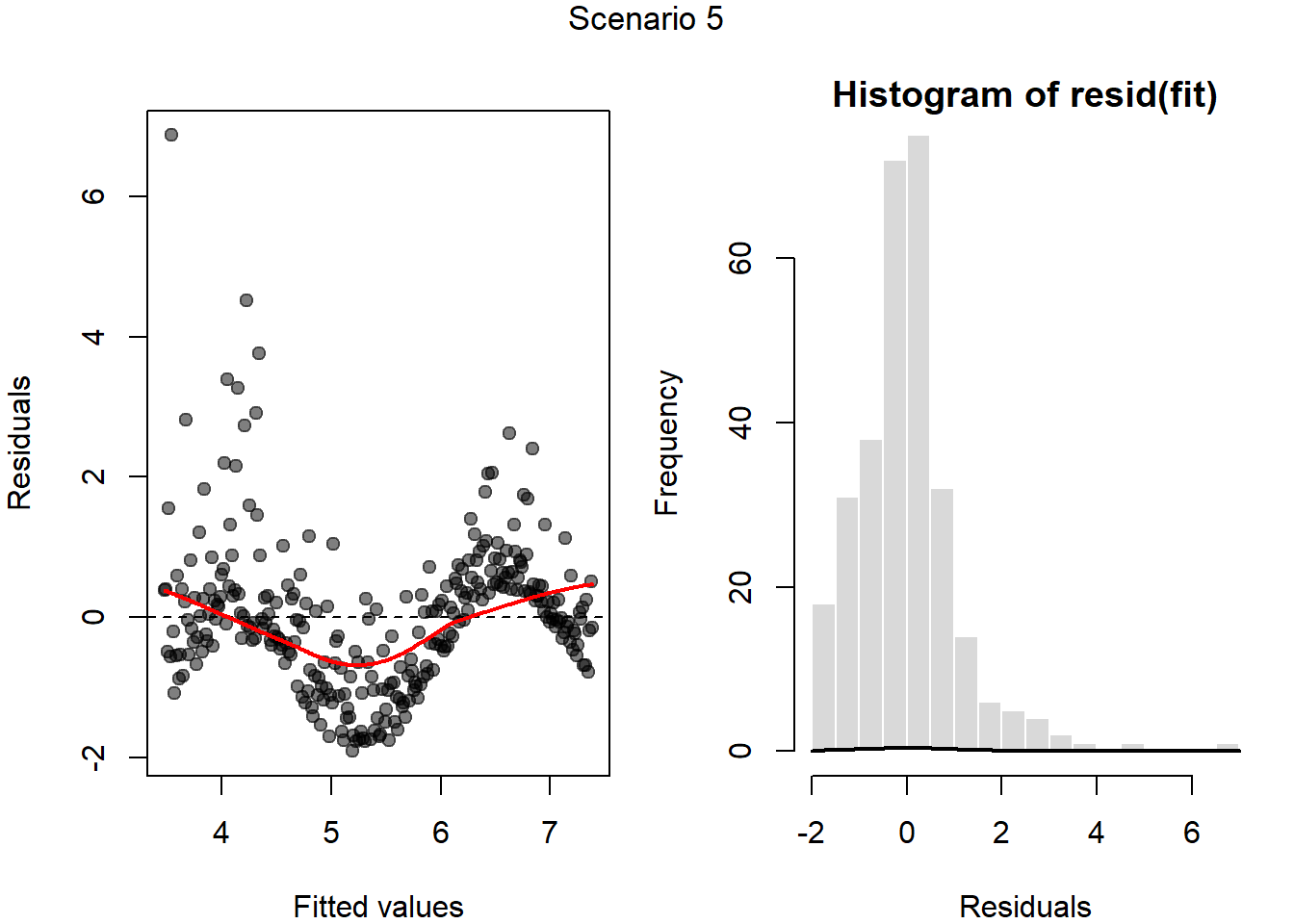
Below are diagnostic plots for assessing assumptions of linear regression for a model. Describe which, if any of the assumptions you would consider might be violated based on these plots
- Scenario 1
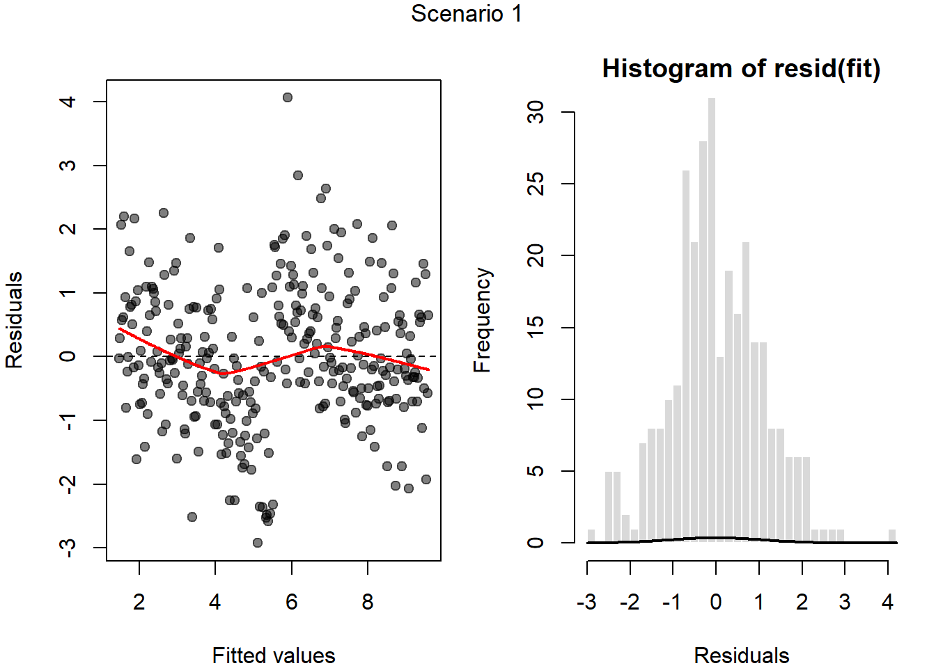
- Scenario 2
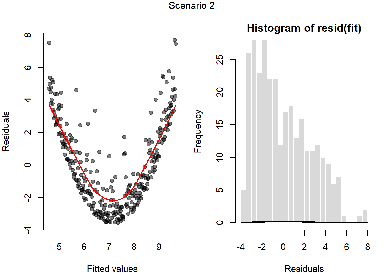
- Scenario 3
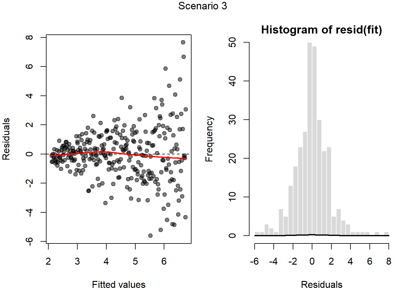
- Scenario 4
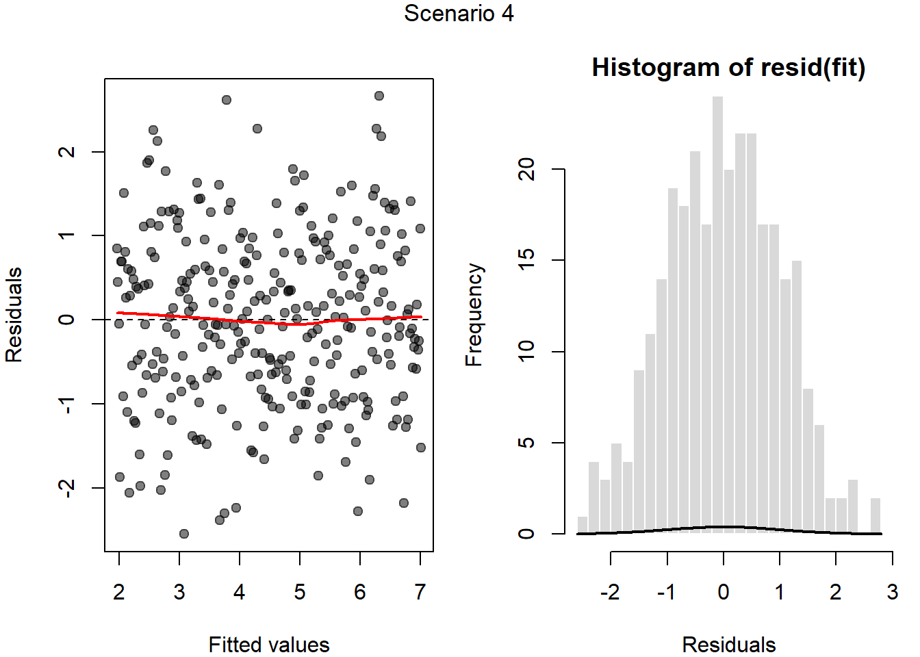
- Scenario 5
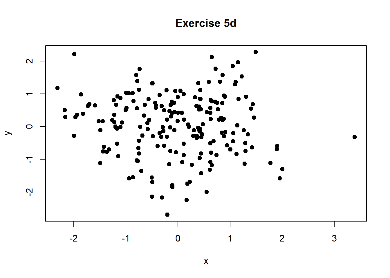
Exercise 5: Correlations
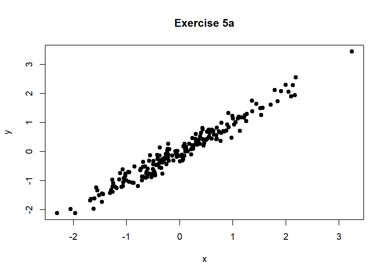
- Describe the direction and strength of the correlation between X and Y in the plot below. Would you expect the Pearson correlation coefficient to be close to 0, close to 1, or somewhere in between?
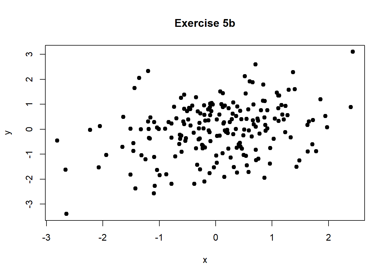
- Describe the direction and strength of the correlation. Would the correlation coefficient be positive or negative?
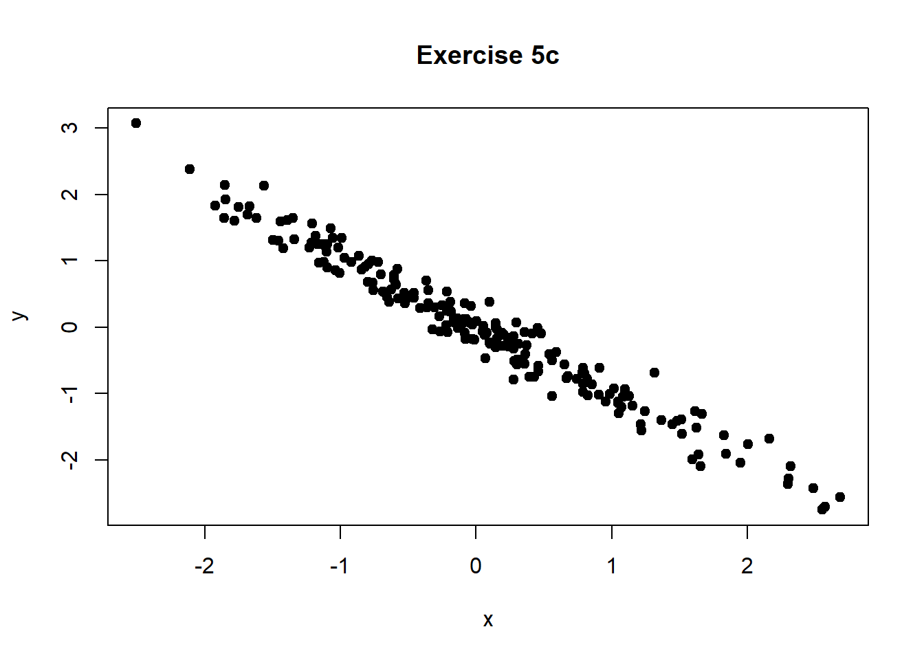
- Is the association between X and Y strong or weak? Would the correlation coefficient be close to 0, close to 1, or close to −1?
- Would you expect the Pearson correlation coefficient to be close to 0, close to 1, or close to −1? Does a correlation near 0 imply there is no relationship between X and Y? Explain briefly.
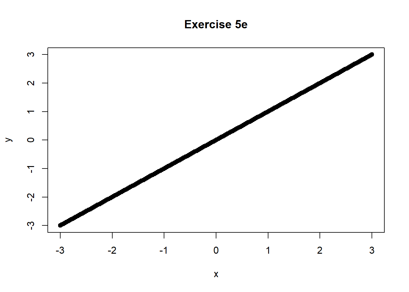
- What value would you expect the correlation coefficient to be close to? How would you describe the relationship between X and Y?
A public health researcher studies the relationship between daily physical activity (minutes per day) and body mass index (BMI) in a community sample and finds that the Pearson correlation coefficient is exactly zero. What does this result tell the researcher about the linear association between physical activity and BMI? Describe a situation in which Spearman correlation would be more appropriate than Pearson correlation for summarizing the association between these two variables. Briefly explain your reasoning.
A public health researcher examines the association between neighborhood air pollution levels (\(PM_{2.5}\) concentration) and lung function (measured by FEV₁) and finds no evidence of a correlation between the two variables based on the Pearson correlation coefficient. However, after controlling for smoking intensity (e.g., pack‑years), the researcher finds that the partial correlation between air pollution and lung function is substantially larger. What does this suggest about the role of smoking intensity in the relationship between air pollution and lung function? Briefly explain how it is possible for the partial correlation to be larger than the unadjusted correlation.
Exercise 6: R Functions and What They Do
For each item in Column A, select the the single best matching description from Column B. Each description should be used exactly once.
Column A: R Functions
cor()
pcor.test()
ggpairs()
lm()
glm(family = "binomial")
predict()
vif()
tidy()
glance()
augment()
Column B: Descriptions
A. Returns a compact summary of overall model fit statistics (e.g., (R^2), F-statistic).
B. Computes variance inflation factors to assess multicollinearity among predictors.
C. Computes a numerical measure of linear association between two numeric variables.
D. Fits a regression model for a binary outcome using a logit link function.
E. Converts model output into a tidy data frame with one row per model coefficient.
F. Generates fitted values or predictions for new or existing observations based on a fitted model.
G. Produces a graphical display showing pairwise relationships among multiple variables.
H. Fits a linear regression model I. Tests the association between two variables while controlling for one or more additional variables.
J. Adds fitted values and residuals to the original dataset for diagnostic purposes.