Solutions: Practice Problems on Collinearity and Logistic Regression

Some of these problems are meant to be fairly difficult–the purpose is to get you to think carefully about the concepts we’ve covered in class, and give you a better understanding of those underlying concepts, in order to be better prepared for the final.

Since some of these are a bit challenging, you are encouraged to discuss these problems in small groups.

Exercise 1: Multicollinearity and linear regression

A (fictional) study examined the association between three air pollutants, Pollutant1, Pollutant2, and Pollutant3, and prevalence of asthma within counties in a fictional U.S. state. The pollutant variables are the average concentrations in parts per billion (ppb) measured at monitoring sites within that county. Prevalence of asthma is the % of the county’s population diagnosed with asthma; it’s treated as normally distributed. The sample comprised 100 counties in this state. Assume hypothesis tests are conducted with significance level \(\alpha=.05.\)


Call:
lm(formula = asthma ~ ., data = df)

Residuals:
   Min     1Q Median     3Q    Max 
-4.968 -1.182  0.130  1.263  5.017 

Coefficients:
            Estimate Std. Error t value Pr(>|t|)    
(Intercept)  7.36391    1.13345   6.497 3.64e-09 ***
Pollutant1  -0.11830    0.17150  -0.690    0.492    
Pollutant2   0.08736    0.16647   0.525    0.601    
Pollutant3   0.10828    0.15910   0.681    0.498    
---
Signif. codes:  0 '***' 0.001 '**' 0.01 '*' 0.05 '.' 0.1 ' ' 1

Residual standard error: 1.971 on 96 degrees of freedom
Multiple R-squared:  0.1202,    Adjusted R-squared:  0.09269 
F-statistic: 4.371 on 3 and 96 DF,  p-value: 0.006261

(a)

What are the results of the hypothesis tests for the significance of each pollutant? Interpret these results in the context of the study.

Each of the hypothesis tests for individual pollutants’ association with asthma prevalence, holding the other pollutant levels constant, have a p-value greater than 0.05. So for each of these tests, we would fail to reject the null hypothesis that the air concentration of that pollutant in ppb is associated with asthma prevalence (%), holding the other pollutant levels constant.

(b)

Write the null and alternative hypotheses for the F-test for overall model significance. Write these hypotheses both in symbols, and in words in the context of the study.

Symbols: \(H_0: \beta_1=\beta_2=\beta_3=0. H_1:\) At least one of \(\beta_j, j=1,2,3\) is not equal to 0. Words: The null hypothesis is that none of the pollutant concentrations (ppb) is associated with asthma prevalence (%). The alternative hypothesis is that at least one of the pollutant concentrations (ppb) is associated with asthma prevalence (%).

(c)

What is the result of the overall F-test for the linear regression model? Interpret this result in the context of the study.

The overall F test results are displayed at the bottom of thee R output summarizing the linear model results, and have a p-value < 0.01, so we reject \(H_0\) and conclude that there is evidence that at least one of the pollutant concentrations (ppb) is associated with asthma prevalence (%).

(d)

Do these results show indication of possible multicollinearity affecting this model? Why or why not?

Yes, one of the typical indications of multicollinearity is that the individual tests are not significant, but the joint test is significant. This occurs because multicollinearity makes it difficult for the linear model to determine, statistically, which predictor variables are individually associated with the response (hence no significant individual associations), but it is still possible to see that at least one of them is associated with the response (joint significance found in the F-test).

(e)

The researchers decide to check for multicollinearity as follows:

library(car)

Loading required package: carData


Attaching package: 'car'

The following object is masked from 'package:dplyr':

    recode

The following object is masked from 'package:purrr':

    some

vif(fit)

Pollutant1 Pollutant2 Pollutant3 
  62.52846   57.92934   53.92988

What did the researchers do? Explain in 1 sentence. What do the results indicate about multicollinearity affecting this model?

The researchers computed the VIF values (variable inflation factor) which checks for multicollinearity. Above 5 or 10 can be considered problematic levels of multicollinearity so it seems to confirm that it is present here.

Exercise 2: Conceptual

Assume the outcome variable \(Y\) takes values either \(0\) or \(1\).

(a)

If our outcome variable \(Y\) takes values \(0\) or \(1\), what would we assume its distribution is?

Bernoulli, or equivalently, binomial with the number of trials equal to 1. We can write this assumption as: \(Y_i\sim Ber(p_i)\).

(b)

We usually want to create a regression model to estimate \(P(Y_i=1)\) based on the value of the predictors for observation \(i\). Thinking back to the properties of the distribution you said in question (a), what is another name for this quantity? In other words, how else can we think of \(P(Y_i=1)\)?

We want to estimate \(P(Y_i=1)\) which in the Bernoulli model we can write as \(p_i\), the parameter for the Bernoulli distribution (for a regression model, the parameter is indexed by \(_i\) because the probability that \(Y_i=1\) depends on the predictor values for that predictor so is different for different observations). The \(Bern(p_i)\) distribution’s expected value is \(p_i\).

(c)

Based on your answer to part (c), how is this similar to the linear regression model with a normally-distributed outcome?

In linear regression where we assume \(Y_i\) is normal, we estimate the expected value of \(Y_i\) given the covariate values, because one way of writing the linear regression assumptions is that \(Y_i\sim N(\beta_0 + \beta_1x_{i1} + ... + \beta_px_{ip}, \sigma^2)\). So in both cases, we are trying to estimate the expected value of the outcome based on the predictor values for that observation. (Note that in logistic regression, we usually write: \(logit(p_i) = \beta_0 + \beta_1x_{i1} + ... + \beta_px_{ip}\), but since the expit function \(expit(x)=\frac{\exp(x)}{1+\exp(x)}\) reverses (“inverts”) the logit function, we can also write the logistic regression model as: \(p_i = expit(\beta_0 + \beta_1x_{i1} + ... + \beta_px_{ip})\). Since \(p_i\) is \(P(Y_i=1)=E(Y_i)\), this hopefully makes it more clear that in both logistic regression and linear regression, we are trying to estimate \(E(Y_i)\) using the predictors for each \(i\), but the models differ due to the use of the logit/expit function in logistic regression.)

(d)

Why would or wouldn’t you want to use a linear regression model for this situation?

The linear regression model assumes a normally distributed outcome, which our outcome variable is not. A normally distributed outcome variable can (hypothetically) take any real number as a value, while our outcome variable must be 0 or 1. So our assumption of normality is incorrect. More concretely, assuming a linear model for the expected value of the outcome, as a function of predictors, can lead to estimated probabilities less than 0 or greater than 1, which are not possible. For these reasons we would not want to use a linear regression model.

(e)

What is the logistic function? Why do we use it in logistic regression?

The logistic or logit function is \(logit(p)=\log\left(\frac{p}{1-p}\right)\). We use it in logistic regression because the logistic model ensures the values of \(p_i\) are always within \([0,1]\) for any predictor values \(x_{i1},...,x_{ip}\).

Specifically, the expit function \(expit(x)=\frac{\exp(x)}{1+\exp(x)}\) takes as input the value of \(\beta_0 + \beta_1x_{i1} + ... + \beta_px_{ip}\), which can be any real number, arbitrarily large or small, and maps that input to an output in \([0,1]\). So the logistic regression model basically takes a linear model, \(\beta_0 + \beta_1x_{i1} + ... + \beta_px_{ip}\), but then applies the expit function to then map the linear part of the model to a probability \(p_i\) that is a valid probability in that it is guaranteed to lie within \([0,1]\).

For the exam, we are looking for you to be able to write the logistic function, and explain that its use in logistic regression is to constrain the estimated probabilities \(p_i\) to lie within \([0,1]\). The extra detail above is just extra explanation.

Exercise 3: Logistic Regression

A (fictional) study examined the association between age (years) and region of residence in the U.S. with diagnosis of a particular condition. They used four regions of the continental U.S., values 1-4.

fit.glm <- glm(condition ~ ., family="binomial", data=df2)
summary(fit.glm)


Call:
glm(formula = condition ~ ., family = "binomial", data = df2)

Coefficients:
             Estimate Std. Error z value Pr(>|z|)    
(Intercept) -9.314872   1.247881  -7.465 8.36e-14 ***
age          0.069713   0.009361   7.447 9.54e-14 ***
BMI          0.248818   0.038797   6.413 1.42e-10 ***
Region2      0.642923   0.361654   1.778   0.0754 .  
Region3      0.542428   0.366574   1.480   0.1389    
Region4      0.821299   0.390035   2.106   0.0352 *  
---
Signif. codes:  0 '***' 0.001 '**' 0.01 '*' 0.05 '.' 0.1 ' ' 1

(Dispersion parameter for binomial family taken to be 1)

    Null deviance: 468.58  on 399  degrees of freedom
Residual deviance: 349.09  on 394  degrees of freedom
AIC: 361.09

Number of Fisher Scoring iterations: 5

(a)

What is the reference category for the region variable? If you wanted to change the reference category, what R command would you use (the one we covered in class)?

Category 1 is the reference category, which we can see because it’s not included as a dummy variable in the R summary output. The function used in class to change the reference category is fct_relevel.

(b)

Write the model used.

Let \(p_i\) be \(P(Y_i=1)\), the probability that individual \(i\) is diagnosed with the condition. Then the model is \(logit(p_i)=\beta_0 + \beta_1 age_i + \beta_2 BMI_i + \beta_3(Region_i=2) + \beta_4(Region_i=3) + \beta_5(Region_i=4)\), where \(Region_i\) can take the values 1, 2, 3, 4 depending on the residence of observation \(i\).

(c)

Conduct a hypothesis test for the association between age and diagnosis probability of the condition, at level \(\alpha=.05\). Follow the steps:

Write the null and alternative hypotheses, in words and symbols.
Compare the p-value to \(\alpha\).
Draw and state your conclusion in the context of the study.

1. \(H_0\): Age (years) is not associated with diagnosis probability, holding region of residence constant. In symbols, \(H_0: \beta_1=0\). \(H_1\): Age (years) is associated with diagnosis probability, holding region of residence constant. In symbols, \(H_1\): \(\beta_1\neq 0\).

2. The p-value is approximately 0, which is less than 0.05, so we reject \(H_0\).

3. We conclude that we have evidence that age (yrs) is associated with probability of diagnosis, holding BMI and region constant.

(d)

Interpret the coefficient for the age variable in the context of the study.

For every increase in age by one year, the odds of diagnosis changes by a factor of \(\exp(\hat{\beta}_1)= \exp(0.069713)\).

(e)

Interpret the coefficient for region category 4 in the context of the study.

Individuals residing in region 4 have odds of diagnosis equal to \(\exp(\hat{\beta}_4)\) times the odds of diagnosis of an individual residing in region 1.

(f)

Based on the sign (positive/negative) of \(\hat{\beta}_1\), is increased age associated with increased or decreased probability of diagnosis?

The sign of the coefficient is positive, meaning that as age increases, the odds of diagnosis increase, and therefore as age increases, probability of diagnosis also increases.

(g)

Suppose the researchers suspect that the association between age and diagnosis probability depends on BMI. They fit the following model.

Given the interaction term is in the model, how do you interpret the coefficient for age?
How do you interpret the p-value for the coefficient for the interaction term?

fit.glm2 <- glm(
  condition ~ age + BMI + age * BMI + Region,
  family = binomial,
  data = df2
)

tidy(fit.glm2) |>
  kable()

term	estimate	std.error	statistic	p.value
(Intercept)	-3.1485524	2.7834083	-1.1311860	0.2579768
age	-0.0693549	0.0590109	-1.1752897	0.2398788
BMI	0.0072106	0.1059317	0.0680686	0.9457310
Region2	0.6299155	0.3643356	1.7289428	0.0838193
Region3	0.5457417	0.3690384	1.4788209	0.1391882
Region4	0.8284514	0.3872593	2.1392680	0.0324140
age:BMI	0.0055405	0.0023506	2.3570612	0.0184202

The coefficient for age is no longer interpretable on its own. We could say that as age increases by one year, the log-odds of diagnosis increase by \(\hat{\beta_1}+\hat{\beta}_6(age_i \times BMI_i)\), where \(\beta_6\) is the coefficient on the interaction term \(age_i \times BMI_i\).

Assuming \(\alpha=0.05\) as above, because the p-value for the interaction term is equal to approximately 0.02 < \(\alpha\), we could conclude that we have evidence for interaction between age and BMI.

Exercise 4: Model Diagnostics

Below are diagnostic plots for assessing assumptions of linear regression for a model. Describe which, if any of the assumptions you would consider might be violated based on these plots

Scenario 1

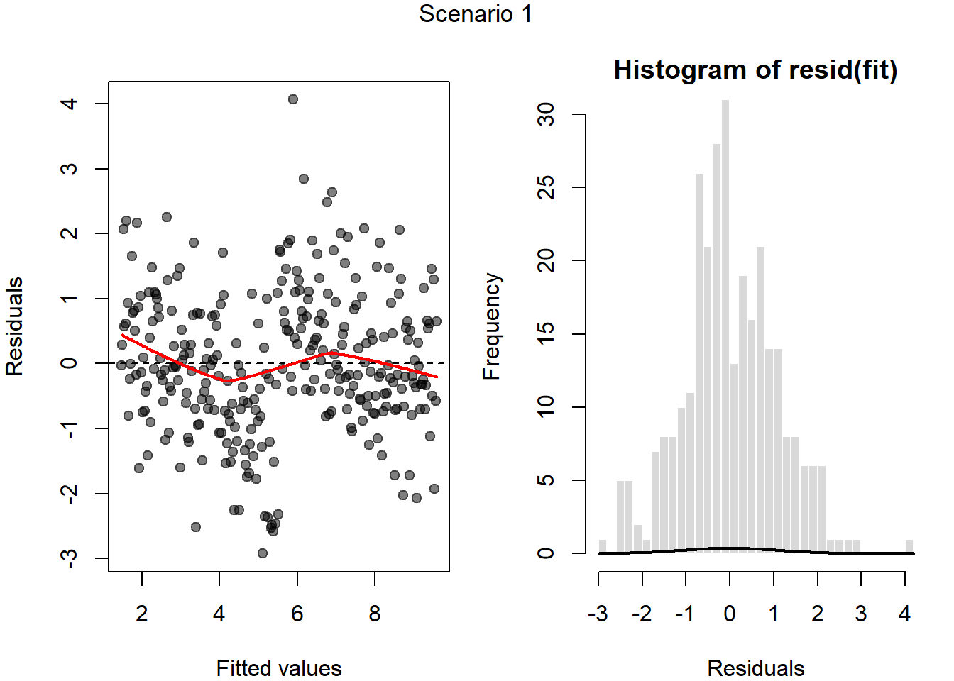
We can see a clear pattern of nonlinearity in the residuals vs. fitted values plot, while we are expecting an even spread of the residuals around 0 if the association is linear, this plot shows a clearp pattern in the spread. The linearity assumption appears violated. The histogram of residuals appears normal.

Scenario 2

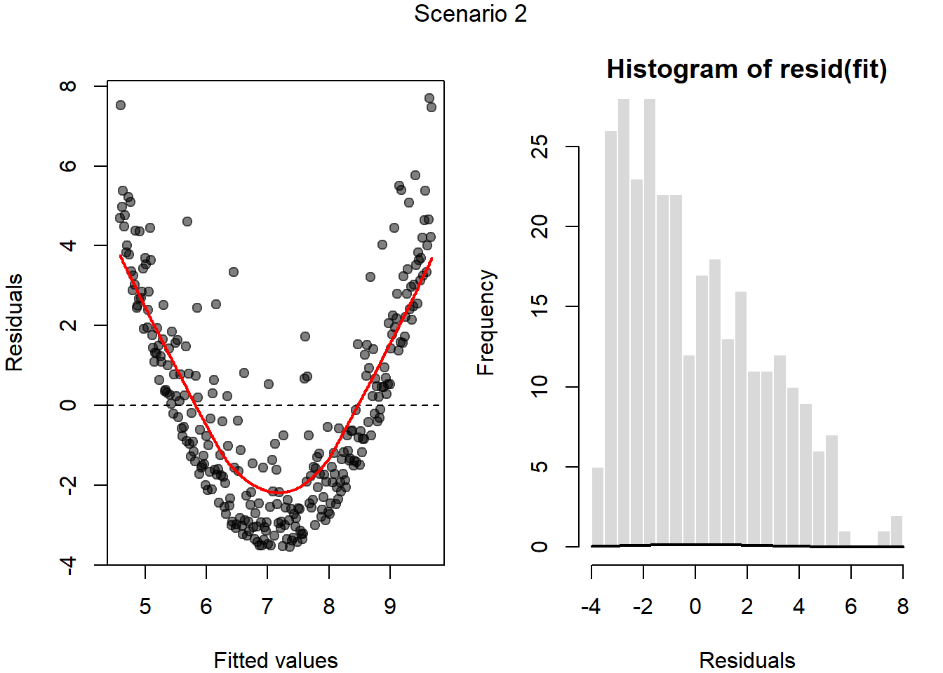
There is clear nonlinearity in the residuals vs. fitted values plot, and the histogram of residuals shows clear departure from normality. The linearity and normality assumptions are both violated.

Scenario 3

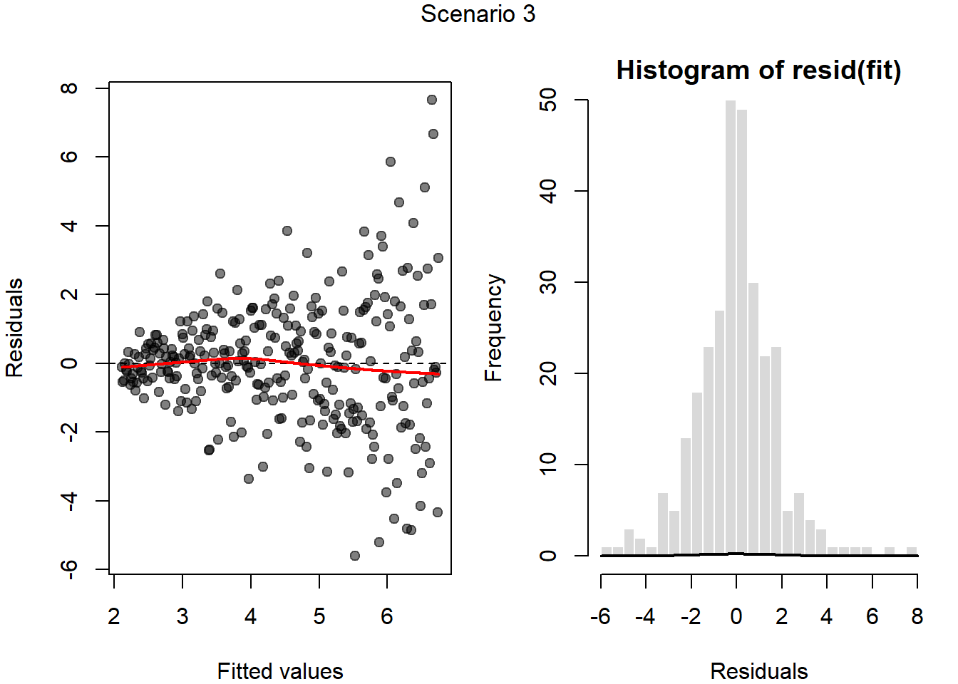
The residuals vs. fitted plot shows the spread of the residuals increasing with the fitted values, indicating that the equal-variances assumption is violated.

Scenario 4

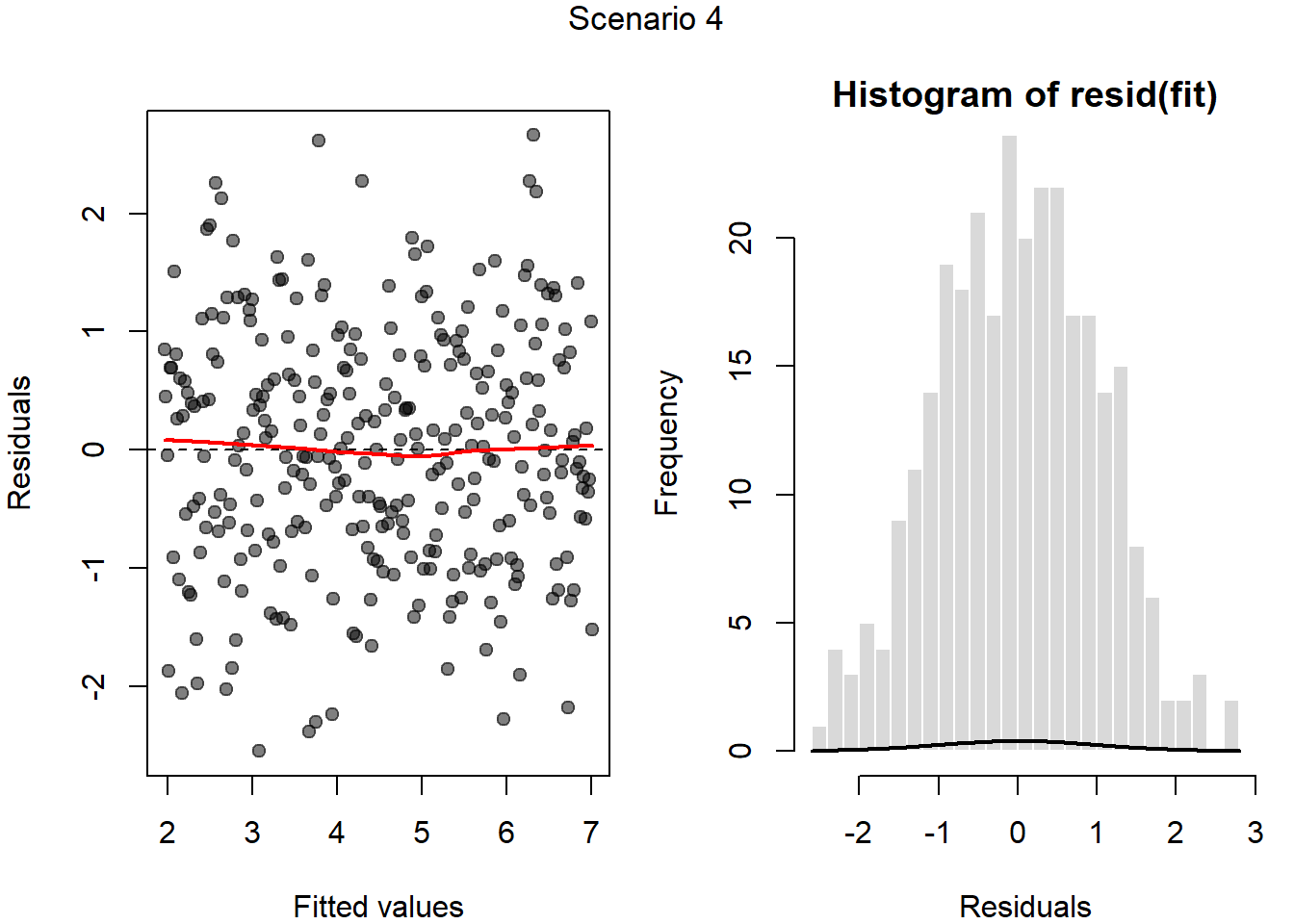
The residuals are evenly spread around the 0 line on the left plot, and appear normal in the right plot, so all assumptions appear reasonable, no violations are apparent.

Scenario 5

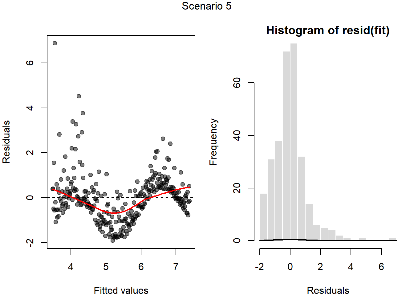
There is clear nonlinearity, unequal variances (larger residuals with lower fitted values), and the residuals appear non-normal in the histogram. Linearity, equal variances, and normality all appear violated.

Exercise 5: Correlations

Describe the direction and strength of the correlation between X and Y in the plot below. Would you expect the Pearson correlation coefficient to be close to 0, close to 1, or somewhere in between?

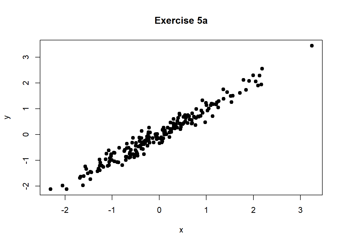
Positive, strong correlation. Close to 1.

Describe the direction and strength of the correlation. Would the correlation coefficient be positive or negative?

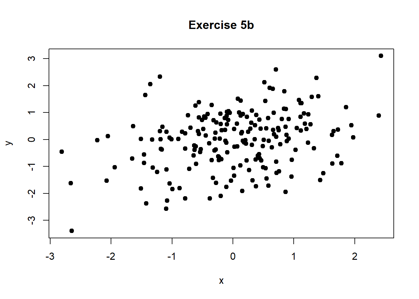
Positive, weak correlation. Coefficient should be positive.

Is the association between X and Y strong or weak? Would the correlation coefficient be close to 0, close to 1, or close to −1?

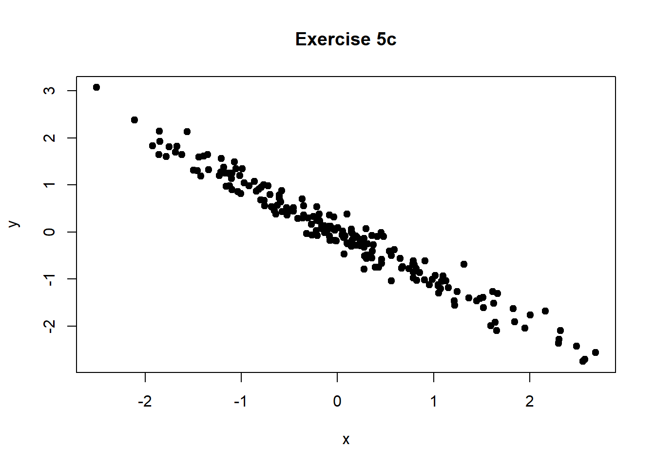
Negative, strong correlation. Close to -1.

Would you expect the Pearson correlation coefficient to be close to 0, close to 1, or close to −1? Does a correlation near 0 imply there is no relationship between X and Y? Explain briefly.

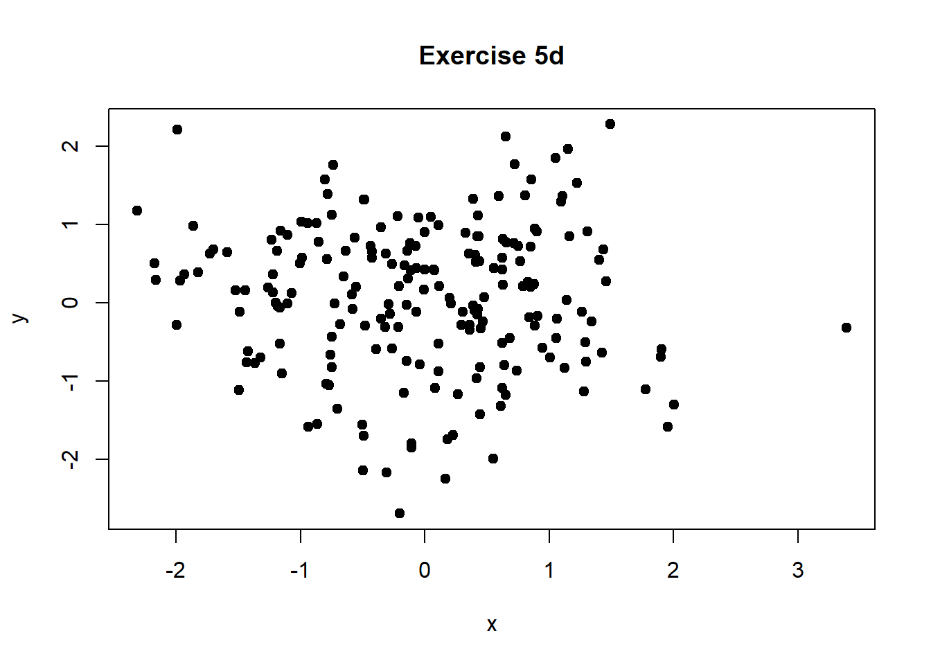
No apparent correlation. Would expect a correlation coefficient near 0. A correlation coefficient near 0 does not alone imply there is no relationship, you would need to look at a scatter plot to confirm there is no relationship, as a nonlinear, nonmonotonic relationship can result in a correlation coefficient near 0.

What value would you expect the correlation coefficient to be close to? How would you describe the relationship between X and Y?

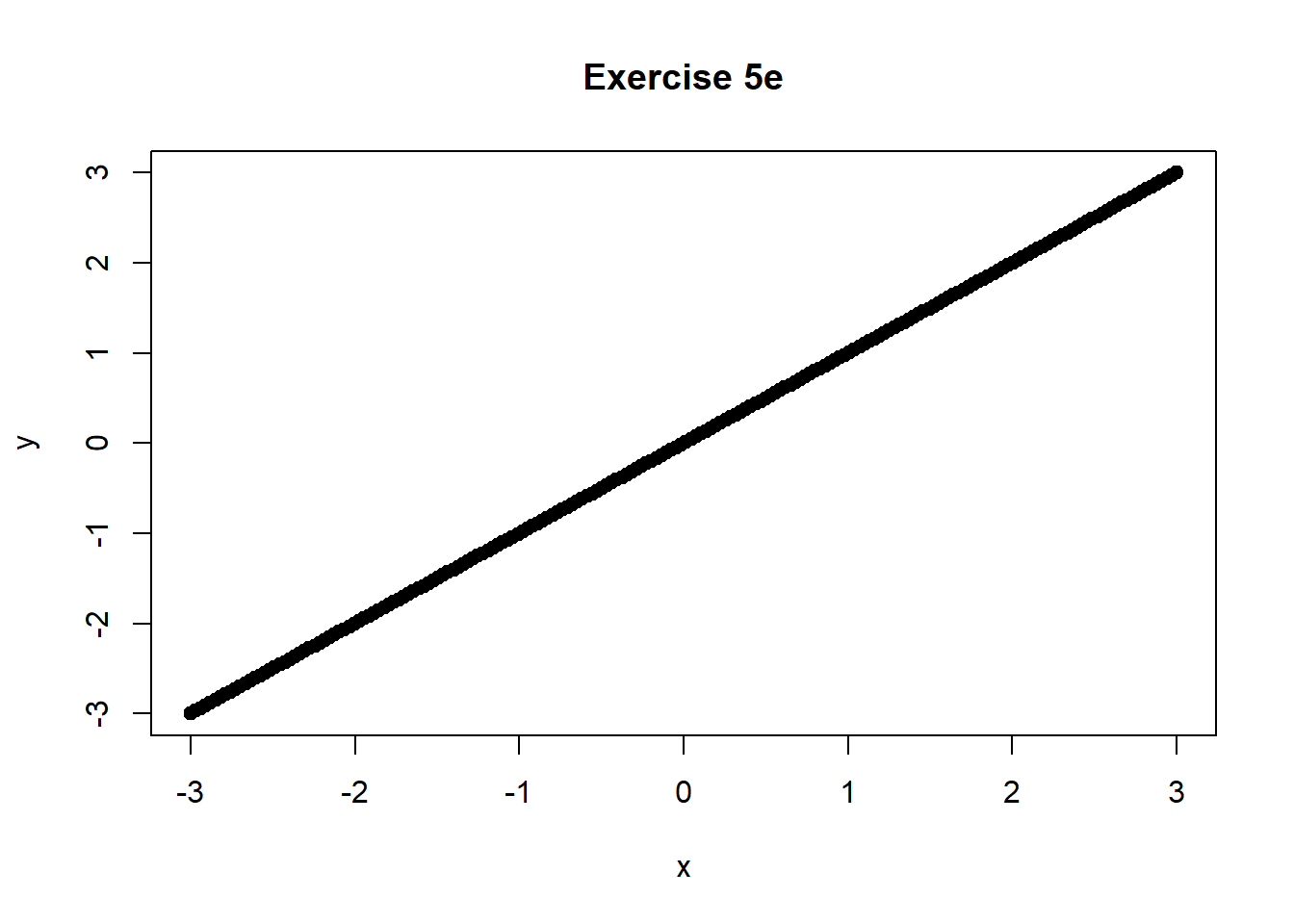
Positive, perfect correlation. Correlation would be equal to 1.

A public health researcher studies the relationship between daily physical activity (minutes per day) and body mass index (BMI) in a community sample and finds that the Pearson correlation coefficient is exactly zero. What does this result tell the researcher about the linear association between physical activity and BMI? Describe a situation in which Spearman correlation would be more appropriate than Pearson correlation for summarizing the association between these two variables. Briefly explain your reasoning.

There is no linear association between daily physical activity (minutes per day) and BMI in this community sample. If the data were plotted in a scatter plot and a nonlinear, but monotone (strictly increasing or decreasing) association was visible, then Spearman correlation would be more appropriate. Spearman correlation does not assume linearity, although it assumes a monotone association.

A public health researcher examines the association between neighborhood air pollution levels (\(PM_{2.5}\) concentration) and lung function (measured by FEV₁) and finds no evidence of a correlation between the two variables based on the Pearson correlation coefficient. However, after controlling for smoking intensity (e.g., pack‑years), the researcher finds that the partial correlation between air pollution and lung function is substantially larger. What does this suggest about the role of smoking intensity in the relationship between air pollution and lung function? Briefly explain how it is possible for the partial correlation to be larger than the unadjusted correlation.

The smoking intensity is a confounding variable. It is associated with both variables, so you need to adjust for smoking intensity to understand the relationship between air pollution and lung function. The partial correlation can be larger than the unadjusted correlation because the true association between air pollution and lung function may only be visible after controlling for the confounding variable

Exercise 6: R Functions and What They Do

For each item in Column A, select the the single best matching description from Column B. Each description should be used exactly once.

Column A: R Functions

cor()
pcor.test()
ggpairs()
lm()
glm(family = "binomial")
predict()
vif()
tidy()
glance()
augment()

Column B: Descriptions

A. Returns a compact summary of overall model fit statistics (e.g., (R^2), F-statistic).
B. Computes variance inflation factors to assess multicollinearity among predictors.
C. Computes a numerical measure of linear association between two numeric variables.
D. Fits a regression model for a binary outcome using a logit link function.
E. Converts model output into a tidy data frame with one row per model coefficient.
F. Generates fitted values or predictions for new or existing observations based on a fitted model.
G. Produces a graphical display showing pairwise relationships among multiple variables.
H. Fits a linear regression model
I. Tests the association between two variables while controlling for one or more additional variables.
J. Adds fitted values and residuals to the original dataset for diagnostic purposes.

1. C 2. I 3. G 4. H 5. D 6. F 7. B 8. E 9. A 10. J