Lecture 10: Hypothesis Testing

BIOS 600 - Spring 2026

Authors

Affiliation

Announcements

Lab 5 materials posted later today, due Sunday March 1 at 11:59pm. No extra grace period!
HW 4 due Thursday at 11:59pm.
Submit exam corrections by Friday, March 6, for up to half your missed points.

Overview

Confidence Intervals Recap
qt() function
Hypothesis tests: how to conduct them, how to interpret them

Confidence Intervals recap

One goal is often estimating a parameter, such as the population mean $\mu$.
We use confidence intervals because they provide a range of plausible values for a parameter, rather than just our best guess.
Form: Point estimate $\pm$ margin of error

Confidence Intervals recap

The margin of error (MOE) is based on a confidence level (such as 95%)
MOE = (confidence multiplier) $\times$ standard error
If we want a higher level of confidence, the confidence multiplier widens the interval

Confidence Intervals recap

In about 95% of random samples, a 95% confidence interval will include the true parameter.
Using that property and the Z-distribution, you can derive the 95% confidence interval starting starting from:

\[ 0.95 = P(-1.96 \leq Z \leq 1.96)\]

Here, 1.96 is the confidence multiplier for a 95% confidence interval based on the standard normal distribution.
You can also find this critical multiplier as the $1-\frac{1-0.95}{2}=0.975$ quantile of the standard normal distribution

Confidence Intervals Recap

When we don’t know the population standard deviation $\sigma$, we can estimate it with the sample standard deviation $s$:

\[ t = \frac{\overline{x}-\mu}{s/\sqrt{n}},\]

but this has a t-distribution with $n-1$ degrees of freedom instead of the $Z$ distribution.

The t-distribution has higher variance, reflecting the fact that we have less information.

Helpful code for HW 4

When constructing a confidence interval with unknown $\sigma$, we need the $t^*$ critical value.
R provides two functions:
- pt() → cumulative probability (area to the left)
- qt() → quantile function (finds cutoff given probability)

Helpful code for HW 4

Example

Suppose we want a 95% confidence interval with $n = 20$ observations:

alpha <- 0.05
n <- 20

# degrees of freedom
df <- n - 1  

# t critical value
t_crit <- qt(1 - alpha/2, df = df)
t_crit

[1] 2.093024

This is the cutoff value such that 95% of the $t_{19}$ distribution lies between $-t$ and $+t$.

Reading

P & G: 10.1 - 10.4
OI: 5.3

Why should we care about hypothesis testing?

How can we answer research questions using statistics?

Statistical hypothesis testing is the procedure that assesses evidence provided by the data in favor of or against some claim about the population (often about a population parameter or potential associations).

The hypothesis testing framework

Start with two hypotheses about the population: the null hypothesis and the alternative hypothesis
Choose a sample, collect data, and analyze the data
Figure out how likely it is to see data like what we got/observed, IF the null hypothesis were true
If our data would have been extremely unlikely if the null claim were true, then we reject it and deem the alternative claim worthy of further study. Otherwise, we cannot reject the null claim

Example: Ultra-low dose contraception

Oral contraceptive pills work well, but must have a precise dose of estrogen.
If a pill has too high a dose, then people may risk side effects such as headaches, nausea, and rare but potentially fatal blood clots
If a pill has too low a dose, pregnancy may occur

Ultra-low dose contraception

A certain contraceptive pill is supposed to contain precisely 0.020 $\mu g$ of estrogen.
During quality control, 50 randomly selected pills are tested, with a sample mean dose 0.017 $\mu g$ and sample SD 0.0008 $\mu g$.

Question

Do you think this is cause for concern? Why or why not?

Two competing hypotheses

The null hypothesis ($H_0$) states that “nothing unusual is happening” / there is no change from status quo / there is no relationship / etc.
The alternative hypothesis ($H_A$ or $H_1$) states the opposite: that there is some sort of relationship (usually this is what we want to check or really think is happening)

Remember, in statistical hypothesis testing we always first assume the null hypothesis is true, and see whether we reject or fail to reject this claim.

Defining the null and alternative hypotheses

Stated in words:

$H_0$: The pills are consistent with a population that has a mean of 0.020 $\mu$g estrogen
$H_1$: The pills are not consistent with a population that has a mean of 0.020 $\mu$g estrogen

Stated in symbols (using LaTeX):

$H_0$: $\mu = 0.020$ renders to —> $H_0$: $\mu$ = 0.020

$H_1$: $\mu \neq 0.020$ renders to —> $H_1$: $\mu \neq$ 0.020

where $\mu$ is the mean estrogen level of the manufactured pills, in $\mu$g.

Collecting and summarizing the data

With these two hypotheses, we now take a sample and summarize the data

The choice of summary statistic calculated depends on the type of data as well as its distribution.
In our example, quality control technicians randomly selected a sample of 50 pills and calculated the sample mean $\bar{x}$ = 0.017 $\mu$g and sample standard deviation $s$ = 0.008 $\mu$g.

Collecting the data in R

(For purposes of this example, we’ve simulated the data with the desired sample size, mean, and sd)

df |>
  slice(1:5)

  sample_data
1  0.01251619
2  0.01515858
3  0.02946967
4  0.01756407
5  0.01803430

Assessing the evidence observed

Next, we calculate the probability of getting data like ours, or more extreme, if $H_0$ were actually true.
This is a conditional probability: “if $H_0$ were true (i.e., if $\mu$ were truly 0.020), what would be the probability of observing statistics like $\bar{x}$ = 0.017 and $s$ = 0.008?”
This probability is the p-value.

Perform one-sample t-test against mu = 0.020

t.test(df$sample_data, mu = 0.020)


    One Sample t-test

data:  df$sample_data
t = -2.6012, df = 49, p-value = 0.01225
alternative hypothesis: true mean is not equal to 0.02
95 percent confidence interval:
 0.01517019 0.01938026
sample estimates:
 mean of x 
0.01727523

Where does -2.6012 come from?

Two-sided tests of hypotheses

To conduct the hypothesis test, we use what we learned about the sampling distribution of the sample mean $\bar{X}$. If the underlying population is normally distributed (or $n$ is pretty large), then the random variable

\[t = \frac{\bar{X}-\mu_0}{s/\sqrt{n}}\]

has a $t_{n-1}$ distribution.

Breaking down the test statistic

\[t = \frac{\bar{X}-\mu_0}{s/\sqrt{n}}\]

$\bar{X} - \mu_0$ tells us how far our sample mean is from the hypothesized population mean

Thus, the test statistic $t$ is an estimate of how many SDs apart $\mu_0$ and $\bar{X}$ are from each other

Let’s calculate our test statistic using the above formula:

Example: Conclusion

If the true average estrogen level really were 0.020 $\mu$g, the chance of seeing data this far off just by random luck is about 1 in 100. (P-value = .01225)
Since that’s very unlikely, we have good evidence the pills’ average estrogen level is not actually 0.020 $\mu$g.
Conclusion: At an alpha level of 0.05, we calculated a p-value of 0.012, which is less than 0.05. There is statistically significant evidence that the mean estrogen level of the manufactured pills is different than 0.020 $\mu$g.
In other words: the pills are probably being made with a slightly different average amount of estrogen than intended.

Getting the p-value graphically (drawing)

Reflection

But wait…

What if $p \geq \alpha$?
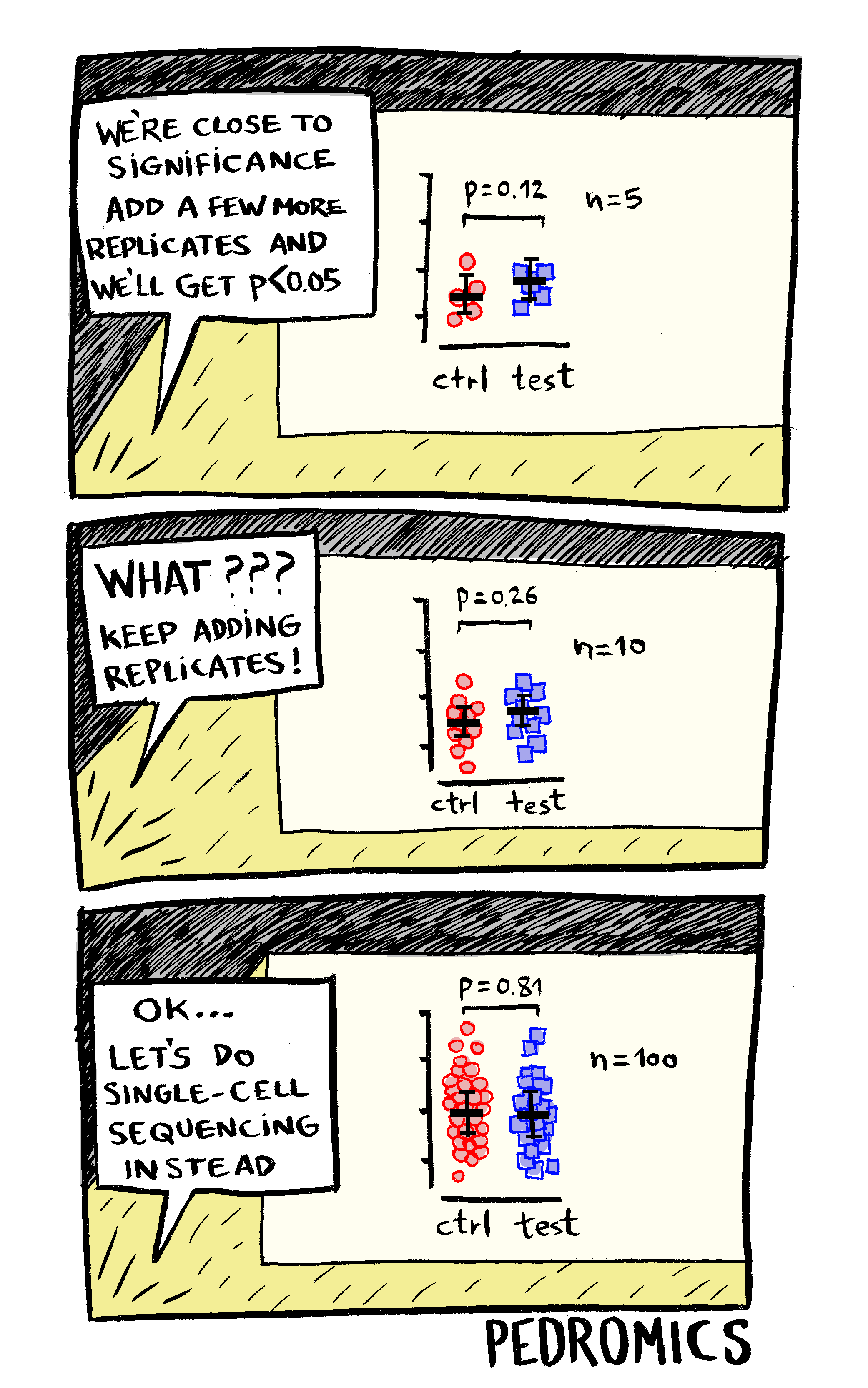
We never “accept” the null hypothesis – we assumed that $H_0$ was true to begin with and assessed the probability of obtaining our test statistic (or more extreme) under this assumption
When we fail to reject the null hypothesis, we are stating that there is insufficient evidence to assert that it is false

Some philosophical details

The obtained p-value relates to the specific test itself, so use of the same data can result in different p-values or confidence intervals depending on which test is used.
Importantly, we have assumed from the start that the null hypothesis is true, and the p-value calculated conditioned on that event.

Caution

p-values do NOT provide information on the probability that the null hypothesis is true given our observed data.

Making a conclusion

We reject the null hypothesis if the conditional probability of obtaining our test statistic, or more extreme, given it is true, is very small
What is “very small”? We often consider a cutpoint (the significance level or $\alpha$ level) defined prior to conducting the analysis
Many analyses use $\alpha = 0.05$: if $H_0$ were in fact true, we would expect to make the wrong decision only 5% of the time (why?)
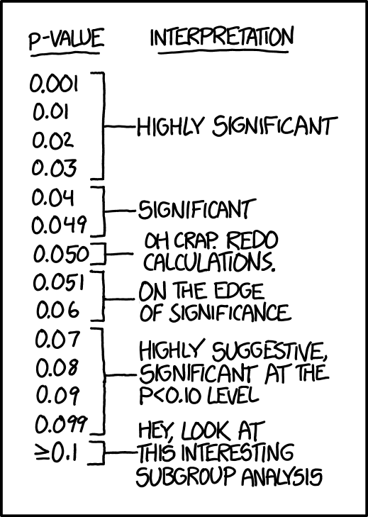
If the p-value is less than $\alpha$, we say the results are statistically significant and we reject the null hypothesis. On the other hand, if the p−value is $\alpha$ or greater, we say the results are not statistically significant and do not reject $H_0$.

What could go wrong?

Suppose we test the null hypothesis $H_0$:$\mu = \mu_0$. We could potentially make two types of errors:

	$\mu = \mu_0$	$\mu \neq \mu_0$
Do not reject $H_0$	correct decision	Type II Error
Reject $H_0$	Type I Error	correct decision

Type I Error: rejecting $H_0$ when it is actually true (falsely rejecting the null hypothesis)
Type II Error: not rejecting $H_0$ when it is false (falsely failing to reject the null hypothesis)

Type I vs. Type II errors

Example: HIV Tests

Type I vs. Type II errors

$H_0$: The patient does not have HIV.

Type 1 error: Test is positive when the person does not have HIV (false positive).
Consequence: Unnecessary stress, stigma, follow-up testing, but not life-threatening if corrected later.
Type II Error: test is negative when person does have HIV (false negative)
Consequence: very serious, patient does not get life-saving treatment, risk of transmission to others.
Therefore, we may design a test to minimize type II error (catch as many true cases as possible), even if that increases false positives?
How about pregnancy tests?

Different sets of hypotheses

We set up the hypotheses to cover all possibilities for $\mu$ and consider three possibilities:

Two-sided: $H_0$:$μ=μ_0$; $H_1$:$μ\neq μ_0$
$H_0$:$μ≥μ_0$; $H_1$:$μ<μ_0$
$H_0$:$μ\leq μ_0$; $H_1$:$μ > μ_0$

Why not use a one-sided test?

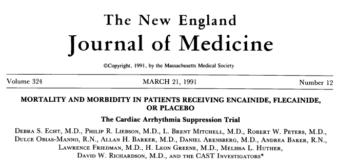
In this study, researchers tested whether anti-arrhythmic drugs (like encainide and flecainide) reduced mortality and morbidity among patients with arrhythmias following a heart attack.
While the initial hypothesis may have been that these drugs would help reduce mortality (a one-sided hypothesis), the study actually found the opposite: the drugs increased mortality rates significantly, leading to the early termination of the trial.

Why a two-sided test is important

Unexpected Adverse Effects: In biomedical research, especially in clinical trials, it’s crucial to remain open to the possibility of unexpected results. A two-sided test accounts for both the potential benefit and harm, ensuring a more balanced and rigorous assessment of treatment effects.
Ethical considerations: Since the primary concern in clinical trials is patient safety, it’s critical to detect any harmful effects early. A one-sided hypothesis test only tests for improvement, which could delay recognizing adverse outcomes.

Recap

qt() function
Hypothesis tests: how to conduct them, how to interpret them
Type 1 and Type 2 error
Why a two-sided test (vs. one-sided) is important

Next class

Comparing two means