library(tidyverse)
licorice <- read.csv("data/licorice.csv")Lecture 11: Comparing Two Means
BIOS 600 - Spring 2026
Announcements
HW 4 due Tonight at 11:59pm.
Lab 5 due Sunday at 11:59pm.
HW 5 will be released after class. HW 5 is due next Thursday March 5 at 11:59pm.
Overview
Review hypothesis test framework
Independent 2-sample t-test vs. paired t-test
Example: independent 2-sample t-test, licorice treatment
Example: paired t-test, exercise plan
Reading
P&G: Chapter 11
OI: 7.3
Review: Hypothesis testing steps
TipFill in the blanks
State the null and alternative hypotheses. The null hypothesis states “____________________________” and the alternative challenges it.
Collect relevant data and summarize it
Assess how surprising it would be to see data like that if the _________________________ were really true
Draw conclusions
Independent samples
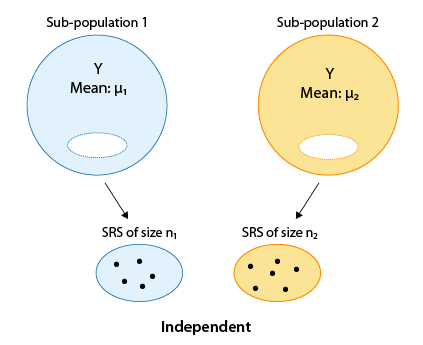
- The type of t-test we use to compare two means depends on how the samples were obtained. One approach would be to obtain two independent samples and test the equality of means \(\mu_1\) and \(\mu_2\)
Paired or matched samples
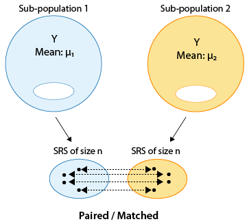
An alternative would be to obtain paired or matched samples and test the equality of means \(\mu_1\) and \(\mu_2\).
Matching could be by person (e.g., before and after measures) or could be a pair of individuals who belong together in another way (e.g., same date of birth in same hospital; married couple, twins etc.)
Paired samples
Samples are often paired for a variety of reasons
Measurements are taken on a single subject at two distinct points in time (e.g., baseline and follow-up)
Subjects may be matched so that members of each pair are as much alike as possible with respect to important characteristics like age and sex (e.g., matched case-control study)
Pairing can control for unwanted sources of variation that might otherwise influence the results of a comparison. Matching within subject (e.g., baseline and follow-up) is a powerful way to eliminate subject-specific factors.
Designing a study: impaired driving
The Department of Motor Vehicles wishes to compare impairment of drivers while texting to impairment after being sleep deprived for 24 hours.
In small groups, describe an independent samples design and a matched pairs design for this question of interest.
Case study: licorice and surgery
Reutzler et al. (2013) performed an experiment among patients having surgery who required intubation.
Prior to anesthesia, patients were randomly assigned to gargle either a licorice-based solution or sugar water (as placebo).
Sore throat was evaluated 30 minutes, 90 minutes, and 4 hours after conclusion of the surgery on a pain scale from 0 to 10 (0 = no pain; 10 = worst).
Let’s evaluate whether gargling licorice before surgery led to different mean pain scores when swallowing, at 30 minutes after arrival in the PACU (post-anesthesia care unit).
Case study: hypothesis testing step 1
- The null hypothesis is that patients receiving licorice gargle (
treat= 1) and sugar solution (treat= 0) placebo have the same mean pain scores relating to swallowing 30 minutes after arrival in the PACU,pacu30min_swallowPain, (treatment is unrelated to mean pain), while the alternative is that they do not.
What are the null and alternative hypotheses written out in symbols?
Setup
- First, we can load tidyverse and read in our data.
Variables of interest:
treat: Treatment given (0 = Sugar placebo; 1 = Licorice solution)pacu30min_swallowPain: Swallow pain score 4 hours after surgery (11-point scale: 0 = No pain; 10 = worst pain)
Looking at some data
licorice |>
  select(pacu30min_swallowPain, treat) |>
  slice(1:5)
pacu30min_swallowPain treat
1 0 1
2 0 1
3 0 1
4 0 1
5 0 1licorice |>
count(treat) treat n
1 0 116
2 1 117Step 2 continued
licorice |>
  group_by(treat) |>
  summarize(mean = mean(pacu30min_swallowPain),
            sd = sd(pacu30min_swallowPain))
# A tibble: 2 × 3
treat mean sd
<int> <dbl> <dbl>
1 0 1.38 2.29
2 1 0.308 0.825Analyzing the data, we obtained
\(\bar{x}_L\)=0.308
\(\bar{x}_S\)=1.38
\(s_L\)=0.825
\(s_S\)=2.29
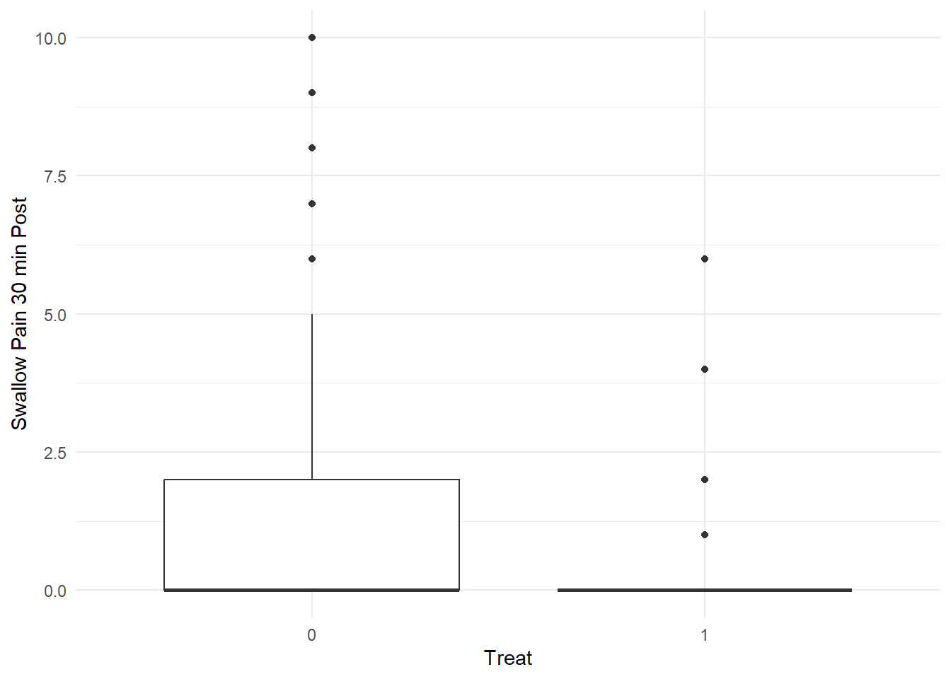
Visualizing the means: code
ggplot(licorice, aes(x = as.factor(treat),
                     y = pacu30min_swallowPain)) +
  geom_boxplot() +
  labs(x = "Treat", y = "Swallow Pain 30 min Post") +
  theme_minimal()
Visualizing the means: plot
Two-sample t-test, independent samples
The two-sample t-test for independent samples is given by
\[t = \frac{(\bar{x}_1 - \bar{x}_2) - (\mu_1 - \mu_2)}{\sqrt{\frac{s_1^2}{n_1} + \frac{s_2^2}{n_2}}}\]
The degrees of freedom of the \(t\) statistic depend on whether or not \(\sigma_1^2 = \sigma_2^2\).
Equal or unequal variances?
The choice of \(df\) depends on whether the independent samples have the same or different variances
If the variances are equal, then we can use a pooled estimate of \(s^2\), and the degrees of freedom are given by \((n_1−1)+(n_2−1)=n_1+n_2−2\).
If the variances are unequal, the degrees of freedom are difficult to derive, and something called a Satterthwaite approximation is often used (use software).
Unequal variances is the default in
t.test()(and it should be the default choice), as the t-test assuming equal variances can be quite unreliable if the variances differ, especially when the group sizes differ as well.
Case study: hypothesis testing step 3
t.test(pacu30min_throatPain ~ treat,
       data = licorice,
       mu = 0,
       alternative = "two.sided",
       var.equal = FALSE,
       conf.level = 0.95)
    Welch Two Sample t-test

data:  pacu30min_throatPain by treat
t = 4.8035, df = 157.3, p-value = 3.608e-06
alternative hypothesis: true difference in means between group 0 and group 1 is not equal to 0
95 percent confidence interval:
 0.4429931 1.0617225
sample estimates:
mean in group 0 mean in group 1
      1.0258621       0.2735043
Case study: hypothesis testing step 3
Carrying out the two sample t-test for independent samples with unequal variances using software on the previous slide, we get \(t=4.80\), \(df\)≈157.3, with a corresponding p-value < 0.001.
Case study: hypothesis testing step 4
- Conclusion: Based on our observed data, we conclude that there is evidence of a potential difference in mean pain score between the two groups. In particular, we have evidence that those receiving the licorice gargle before their surgery reported a lower mean pain score compared to placebo patients.

Case study: athletic training
- A school athletics department wants to test the effectiveness of the new type of training proposed by comparing the average times of 10 runners in the 100 meters in seconds before and after the new training is implemented.
What are \(H_0\) and \(H_1\)?
Which test should we use?
In R
- Our dataset in R is called
training:
training subject before after
1 1 12.9 12.0
2 2 13.5 12.2
3 3 12.8 11.2
4 4 15.6 13.0
5 5 17.2 15.0
6 6 19.2 15.8
7 7 12.6 12.2
8 8 15.3 13.4
9 9 14.4 12.9
10 10 11.3 11.0Paired t-test
t.test(training$before,
       training$after,
       mu = 0,
       paired = T,
       alternative = "two.sided",
       var.equal = FALSE,
       conf.level = 0.95)
    Paired t-test

data:  training$before and training$after
t = 5.2671, df = 9, p-value = 0.0005158
alternative hypothesis: true mean difference is not equal to 0
95 percent confidence interval:
 0.9185294 2.3014706
sample estimates:
mean difference
           1.61
Conclusion
Tip
What is your conclusion?
But wait…
training_diff <- training |>
  mutate(diff = after - before)
training_diff
subject before after diff
1 1 12.9 12.0 -0.9
2 2 13.5 12.2 -1.3
3 3 12.8 11.2 -1.6
4 4 15.6 13.0 -2.6
5 5 17.2 15.0 -2.2
6 6 19.2 15.8 -3.4
7 7 12.6 12.2 -0.4
8 8 15.3 13.4 -1.9
9 9 14.4 12.9 -1.5
10 10 11.3 11.0 -0.3But wait..
t.test(training_diff$diff,
       mu = 0,
       alternative = "two.sided",
       conf.level = 0.95)
    One Sample t-test

data:  training_diff$diff
t = -5.2671, df = 9, p-value = 0.0005158
alternative hypothesis: true mean is not equal to 0
95 percent confidence interval:
 -2.3014706 -0.9185294
sample estimates:
mean of x
    -1.61
Takeaway
- A paired t-test is the same as a one-sample t-test on the differences.
Recap
Review hypothesis test framework
Independent 2-sample t-test vs. paired t-test
Example: independent 2-sample t-test, licorice treatment
Example: paired t-test, exercise plan
Next class
- Thursday’s class: ANOVA