Lecture 14: Non-Parametric tests

BIOS 600 - Spring 2026

Announcements

Lab 7: after break/exam.
Tuesday, March 31: Exam 2
HW6: due Thursday after break (3/26).

Very optional reading

P&G Chapters 13
OI: Sections 8.1

Overview

Nonparametric methods
Sign test, Wilcoxon signed-rank test, Wilcoxon rank-sum test
Krustal-Wallis test

Why nonparametric methods?

For the methods we have studied so far, we have assumed the populations from which the data were drawn were either normally distributed or approximately so. This is a necessary property for the tests to be valid.
Because the distributional form is assumed known, with only values of \(\mu\) and \(\sigma\) unknown, these methods are known as parametric methods.
Nonparametric methods make fewer assumptions about the nature of the underlying distributions and may be appropriate when some assumptions of parametric methods are not satisfied.

Sign test

The sign test is a nonparametric alternative to the paired t-test. It does not assume normality but just requires that observations are independent.
The null hypothesis of the sign test is that the median difference among pairs in the underlying population is 0.

Sign test: cold data

A medical researcher claims that a new vaccine will decrease the number of colds in adults.
You randomly select 14 adults and record the number of colds each has in a one-year period.
After giving the vaccine to each adult, you again record the number of colds each has in a one-year period.
At \(\alpha = 0.05\), do the data support the researcher’s claim?

# Colds
Before	3	4	2	1	3	6	4	5	2	0	2	5	3	3
After	2	1	0	3	1	3	3	2	2	2	2	3	4	3

Sign test

The sign test has just a few simple steps:

Take the difference of each pair of observations (e.g., before-after)
Record the sign of each difference (+, –, or 0)
Count the number of + signs
Test using the binomial distribution with \(n =\) number of pairs with nonzero differences and \(p=0.5\), as we would expect the same number of positive and negative signs under \(H_0\).

Sign test

The differences do NOT look very normal and we have a relatively small sample size. So, we cannot use previous methods to solve this question (and must rely on the sign test)!

# Colds
Before	3	4	2	1	3	6	4	5	2	0	2	5	3	3
After	2	1	0	3	1	3	3	2	2	2	3	4	3	2
Diff.	1	3	2	-2	2	3	1	3	0	-2	-1	1	0	1
Sign	+	+	+	–	+	+	+	+	0	–	–	+	0	+

12 non-zero differences, with 9 + signs

Sign test for cold data

\(H_0\): Median difference in colds = 0 (i.e. same number of positive and negative signs)

\(H_A\): Median difference in colds \(\neq\) 0 (i.e. different number of positive and negative signs)

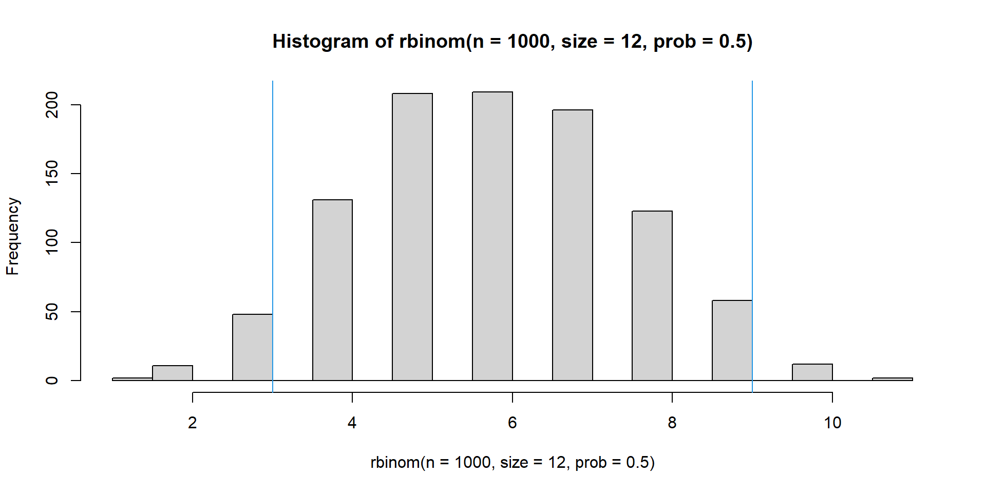
Remember, we had 9 successes out of 12 trials.
What is the probability we see 9 successes out of 12 trials in a binomial distribution (or more extreme, in either direction), if the null hypothesis that \(p=0.5\) is true?

Conducting the sign test

We can calculate, for \(X\sim Binom(12,0.5)\),

\(P(X=9) + P(X=10) + P(X=11) + P(X=12)\)

and then double it (for the two-sided test).

hist(rbinom(n=1000,size=12,prob=.5),breaks=30)
abline(v=9, col=4)
abline(v=3, col=4)

2*(1-pbinom(8, 12, 0.5))

[1] 0.1459961

Conducting the sign test

Conclusion: With p = .145, we fail to reject \(H_0\) and hence conclude that there is not enough evidence to suggest there is a difference in the median number of colds in the years before and after vaccine administration.

Wilcoxon signed-rank test

The sign test is appealing because it avoids all distributional assumptions. However, it ignores the magnitude of the differences.
If we are willing to assume that the differences are symmetrically distributed around the median, we can incorporate the magnitude of the differences and gain considerable power using the Wilcoxon Signed-Rank Test.
The Wilcoxon signed-rank test is an alternative to the paired t-test. The \(H_0\) is that the median difference in the underlying population is 0.

Rank-based methods

Many non-parametric methods have a similar flavor to parametric methods but are computed on the ranks instead of the observed data.
The rank of an observation, among a set of observations, is its position when the observations are ordered from smallest to largest. The smallest observation has rank 1, next smallest has rank 2, and so forth.
If observations are tied, the rank assigned to each is the average of the ranks appropriate to the equal numbers.

Why ranks?

Using the ranks provides robustness against outliers:

X: 175, 169, 190
- Ranks: 2, 1, 3
X: 175, 169, 490
- Ranks: 2, 1, 3 (robust to outlier)
X: 175, 175, 190
- Ranks: 1.5, 1.5, 3 (take sum of ranks and divide by number tied)

Wilcoxon signed-rank test

Like the sign test, the Wilcoxon signed-rank test is for paired differences and has just a few simple steps:

Calculate the difference for each pair of observations
Rank the absolute values of these differences from smallest to largest (drop 0’s; assign an average rank to ties); let \(n\) be the number of non-zero differences
Assign each rank a + or – depending on the original sign of the difference
Add up all positive ranks; add up all negative ranks; let \(T\) be equal to the smaller sum

Wilcoxon signed-rank test

Calculate the z-score

\[z_T = \frac{T - \frac{n(n+1)}{4}}{\sqrt{\frac{n(n+1)(2n+1)}{24}}}\]

and obtain a p-value from the normal distribution.

Don’t do this by hand – we will use R.

Example: middle ear effusion

A common symptom of otitis media in young children is the prolonged presence of fluid in the middle ear, known as middle-ear effusion. The presence of fluid may result in temporary hearing loss and interfere with normal learning skills in the first 2 years of life.
One hypothesis is that babies who are breastfed for at least one month build some immunity and have less prolonged effusion than their bottle-fed counterparts.
A small study of 14 babies is set up, with babies matched one-to-one by age, sex, socioeconomic status, and health condition. One member of the pair is a breastfed baby, and the other member is a bottle-fed baby. The outcome is the duration (days) of middle-ear effusion after the first episode of otitis media.

Example: middle ear effusion

Duration of Effusion for Each Pair (Days):

Pair	1	2	3	4	5	6	7	8	9	10	11	12	13	14
Breast	26	3	12	28	7	39	12	30	7	15	65	10	19	11
Bottle	18	7	6	33	7	57	29	28	8	27	78	17	16	35

Question

What is \(H_0\)?

Example: middle ear effusion

Duration of Effusion for Each Pair (Days):

	1	2	3	4	5	6	7	8	9	10	11	12	13	14
Breast	26	3	12	28	7	39	12	30	7	15	65	10	19	11
Bottle	18	7	6	33	7	57	29	28	8	27	78	17	16	35
Diff	8	-4	6	-5	0	-18	-17	2	-1	-12	-13	-7	3	-24
Abs. Diff	8	4	6	5	0	18	17	2	1	12	13	7	3	24
Rank	8	4	6	5	NA	12	11	2	1	9	10	7	3	13
Signed Rank	8	-4	6	-5	NA	-12	-11	2	-1	-9	-10	-7	3	-13

Sum of positive ranks is smaller than sum of negative ranks
Sum of positive ranks = 8 + 6 + 2 + 3 = 19 = \(T\)
\(z_T = \frac{19-\frac{13(14)}{4}}{\sqrt{\frac{13(14)(27)}{24}}} = \frac{19-45.5}{3} = -1.85\) \(\rightarrow\) Now, let’s calculate our p-value.

Calculating the p-value

zt <- (19-(13*14/4))/sqrt(13*14*27/24)
zt

[1] -1.85197

pnorm(zt)*2 # two-sided test

[1] 0.06403015

Conclusion: With \(p > 0.05\), we fail to reject the null hypothesis. We do not have sufficient evidence to suggest that there is a difference in the median of the paired differences in effusion duration between being breast and bottle-fed.

Wilcoxon rank sum test

Not to be confused with the Wilcoxon Signed-Rank Test!

The Wilcoxon Rank Sum Test:

Is the non-parametric counterpart of the two-sample t-test
Assumes two samples are independent but does not require normality or equal variance of groups
Assumes two distributions have “roughly the same shape”
Also called the Mann-Whitney U test or Wilcoxon-Mann-Whitney test

Mann-Whitney U test

The Mann-Whitney U-test is an extension of the Wilcoxon signed rank test for independent samples.
Instead of taking differences, the observations are lumped together and ranked, with then the sum of the ranks calculated by group.
We’ll use software to perform this test.

Example: Exercise capacity and coronary artery disease

Consider data from a two-group study of exercise capacity.
Two groups of men, one with diagnosed three-vessel coronary artery disease (3VD), and the other group of men with suspected disease (SD) in one or more vessels.
The total time participants could exercise on a treadmill set to increase in speed and slope according to a set schedule, is below:
3VD times: 864, 636, 638, 708, 786, 600, 1320, 750, 594, 750
SD times: 1014, 684, 810, 990, 840, 978, 1002, 1110
3VD median: 729
SD median: 984

Example: Exercise capacity and coronary artery disease

Value	Rank	Group	Value	Rank	Group
594	1	3VD	810	10	SD
600	2	3VD	840	11	SD
636	3	3VD	864	12	3VD
638	4	3VD	978	13	SD
684	5	SD	990	14	SD
708	6	3VD	1002	15	SD
750	7.5	3VD	1014	16	SD
750	7.5	3VD	1110	17	SD
786	9	3VD	1320	18	3VD

Sum of ranks in SD group, \(n=8\): 101
Sum of ranks in 3VD group, \(n=10\): 70

Example

The sum of the ranks in the SD group with \(n=8\) was 101, and the 3VD group had 10 subjects with sum of ranks 70. Is this enough evidence to reject the null hypothesis?

Mann-Whitney U Test Statistic

Group	n	Sum of Ranks
SD	8	101
3VD	10	70

Step 1 Compute U-statistics.

\[U_1 = R_1 - \frac{n_1(n_1+1)}{2}, \quad U_2 = R_2 - \frac{n_2(n_2+1)}{2}\]

where \(R_1\) and \(R_2\) are the sums of ranks in groups 1 and 2, respectively, and \(n_1\) and \(n_2\) are group sample sizes.

Step 2 Either \(U_1\) or \(U_2\) can be used as the test statistic \(U\).

U-statistic

When both sample sizes are \(\geq 8\), the sampling distribution of U is approximately normal with mean and standard deviation:

\[\text{mean}_U = \frac{U_1 + U_2}{2} = \frac{n_1 n_2}{2}, \quad \text{sd}_U = \sqrt{\frac{n_1 n_2 (n_1 + n_2 + 1)}{12}}\]

In other words, \(U_1 + U_2 = n_1 \cdot n_2\), so once you know one, you automatically know the other.
If there are ties, the standard deviation uses a different formula.

No need to memorize this!

In R

# Given data
n1 <- 8; n2 <- 10
R1 <- 101; R2 <- 70

U1 <- R1 - n1 * (n1 + 1) / 2
U2 <- R2 - n2 * (n2 + 1) / 2
U1; U2

[1] 65

[1] 15

In R

mean_U <- n1 * n2 / 2
sd_U <- sqrt(n1 * n2 * (n1 + n2 + 1) / 12)
z <- (U1 - mean_U) / sd_U
p_value <- 2 * (1 - pnorm(z))

z; p_value

[1] 2.221308

[1] 0.02633009

As it turns out, we reject \(H_0\) and conclude the two groups do not have the same median. The median exercise time in the SD group is higher compared to the 3VD group.

Why do we use \(U_1\) when computing \(z\)?

When approximating the test statistic using the normal distribution:

\[z = \frac{U - \text{mean}_U}{\text{sd}_U}\]

you can use either \(U_1\) or \(U_2\) - they’ll lead to the same p-value once you take into account the direction of the test.

By convention, we usually use \(U_1\), the statistic associated with the first group.
Using \(U_1\) or \(U_2\) would yield the same absolute z-score, since \(U_1\) and \(U_2\) are complements.

Check

Using \(U_2\):

z <- (U2 - mean_U) / sd_U
p_value <- 2 * (pnorm(z))

z; p_value

[1] -2.221308

[1] 0.02633009

We see that our \(z\) value is simply the negative of the previous \(z\) value. Using a two-sided test, we get the same p-value.

Note

Alternative way of calculating p-value

Note that we can also calculate our p-value using:

2 * pnorm(-abs(z))

[1] 0.02633009

Why can we do this? Can you draw a picture to explain why these two methods yield the same result? (Look up ?abs in the Console)
Why might this code be more generalizable compared to the previous code to calculate the p-value?

Kruskal-Wallis test

The Kruskal-Wallis Test is the nonparametric version of ANOVA, generalizing the Wilcoxon rank sum test to more than 2 groups.

Kruskal-Wallis test for pet data

Consider the study of pulse rate from the ANOVA lecture.
Remember that pulse rates were not necessarily normally distributed within groups.

Kruskal-Wallis test for pet data

Calculating the sum of the ranks, we find that in the pet group, out of \(n=30\), the sum of the ranks was 863; out of the \(n=30\) in the friend group, the sum of the ranks was 1797, and out of the \(n=30\) where neither were present, the sum of the ranks was 1435. Is this enough evidence to reject the null hypothesis? (Ask software).

kruskal.test(pulse ~ group, data = pulse_data)


    Kruskal-Wallis rank sum test

data:  pulse by group
Kruskal-Wallis chi-squared = 21.662, df = 2, p-value = 1.978e-05

The p-value is < 0.0001. What may we conclude?

Pairwise comparisons: pet vs. friend

Again, we can step-down and look at pairwise differences. In this case, we would use the Wilcoxon Rank-Sum test (why?).

🧪 When to Use Kruskal–Wallis vs. ANOVA

Feature	One-Way ANOVA	Kruskal–Wallis Test
Purpose	Tests whether the means of 3+ groups differ	Tests whether the distributions (typically medians) differ
Data type	Continuous, roughly normal	Ordinal or continuous, not normal
Assumptions	1. Normality within groups 2. Equal variances (homoscedasticity) 3. Independent samples	1. Independent samples 2. Same-shaped distributions (for median interpretation)
Basis of test	Uses group means and within-group variance	Uses ranks of data instead of raw values
Example use	Compare mean blood pressure across 3 treatment groups	Compare pain severity scores (on a 0–10 scale) across 3 treatment groups when scores are skewed

Quick Intuition

Use ANOVA if your data meet parametric assumptions (normal, equal variances).
Use Kruskal–Wallis if your data are skewed, ordinal, or have outliers that violate ANOVA’s assumptions.

Why not always go nonparametric?

Non-parametric methods are desirable because they do not require as many restrictive assumptions as parametric ones.
However, this flexibility comes at a price – if the assumptions underlying a parametric test are satisfied, the nonparametric test is less powerful than the comparable parametric technique. We’ll talk about statistical power next class.

Next Class

Power and sample size calculation (incredibly useful!)