Lecture 16: Comparing two continuous variables
BIOS 600 - Spring 2026
Announcements
HW 6 Due Thursday at 11:59pm. Will be graded by the end of the weekend.
No new lab this week, the session at 3:30pm is just TA Office Hours.
Exam 02 is in-class on Tuesday, March 31.
Thursday’s class will be review for exam.
Next new lab will be after the exam.
Exam 02 Info
Practice problems will be posted today
Formula sheet, topic list on course website
Nonparametric methods vs parametric methods
| Parametric test | Nonparametric test |
|---|---|
| Paired/one-sample t-test | Sign test |
| Paired/one-sample t-test | Signed rank test |
| Two-sample t-test | Rank sum test (aka Mann Whitney U test) |
| ANOVA | Kruskal-Wallis |
Reading
P&G Chapter 17
OI: Section 8.1
Motivation: Comparisons of Interest
| Predictor Type | Outcome Type | Common Tests / Topics |
|---|---|---|
| Categorical | Categorical | Fisher’s exact test, \(\chi^2\) test |
| Categorical | Continuous | t-tests, ANOVA, nonparametric alternatives |
| Continuous | Continuous | Correlation*, regression ** |
| Continuous | Categorical | Logistic regression, classification ** |
| Other / Complex | Various (e.g. survival, counts) | Advanced or “exotic” methods ** |
* = covering today
** = covering in upcoming lectures
Remember this plot?
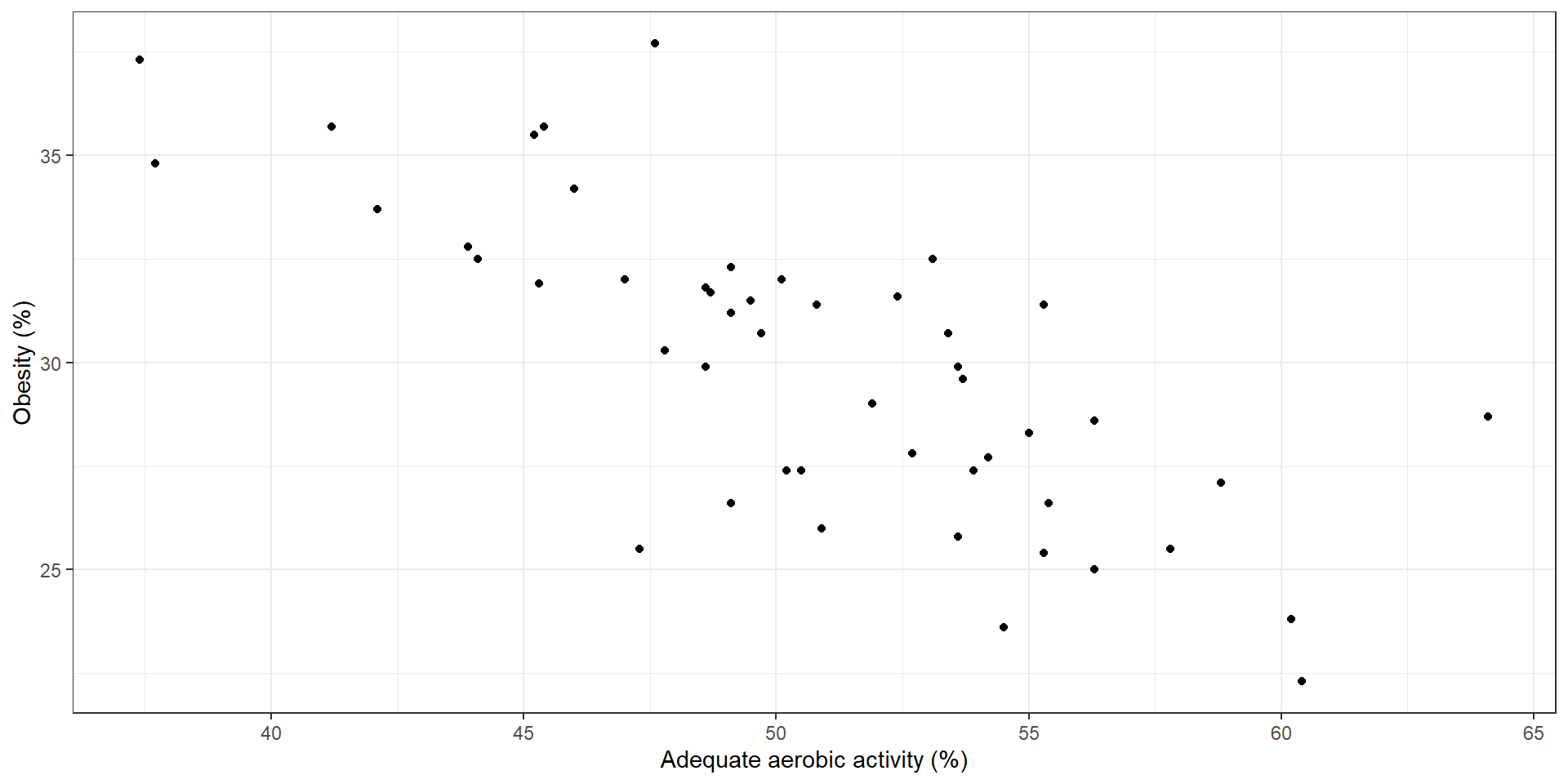
Some questions of interest may include:
Direction of relationship: are variables positively or negatively related?
Form: is any relationship linear or more complex?
Strength of relationship: how accurately can one variable predict the other?
Influential points: are one or a few points driving the relationship we see?
Correlation
The correlation coefficient \(\rho\) quantifies the linear relationship between two random variables.
In statistics, a correlation coefficient implies a very specific type of association.
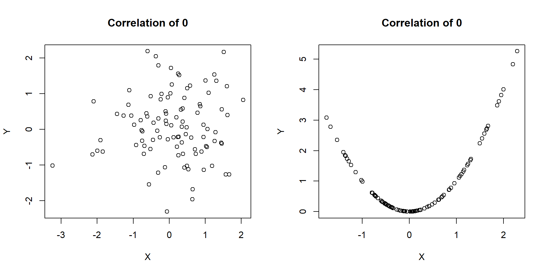
A correlation coefficient of zero does NOT imply no relationship between two variables, as we shall see in some further examples.
Correlation
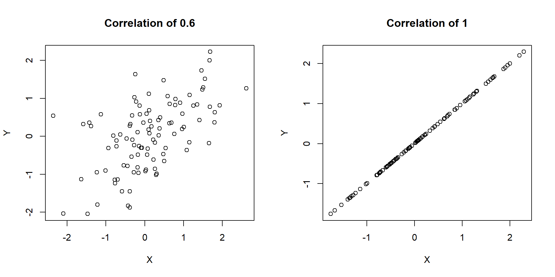
\(\rho\) ranges from -1 to 1
\(\rho>0\) implies positive correlation
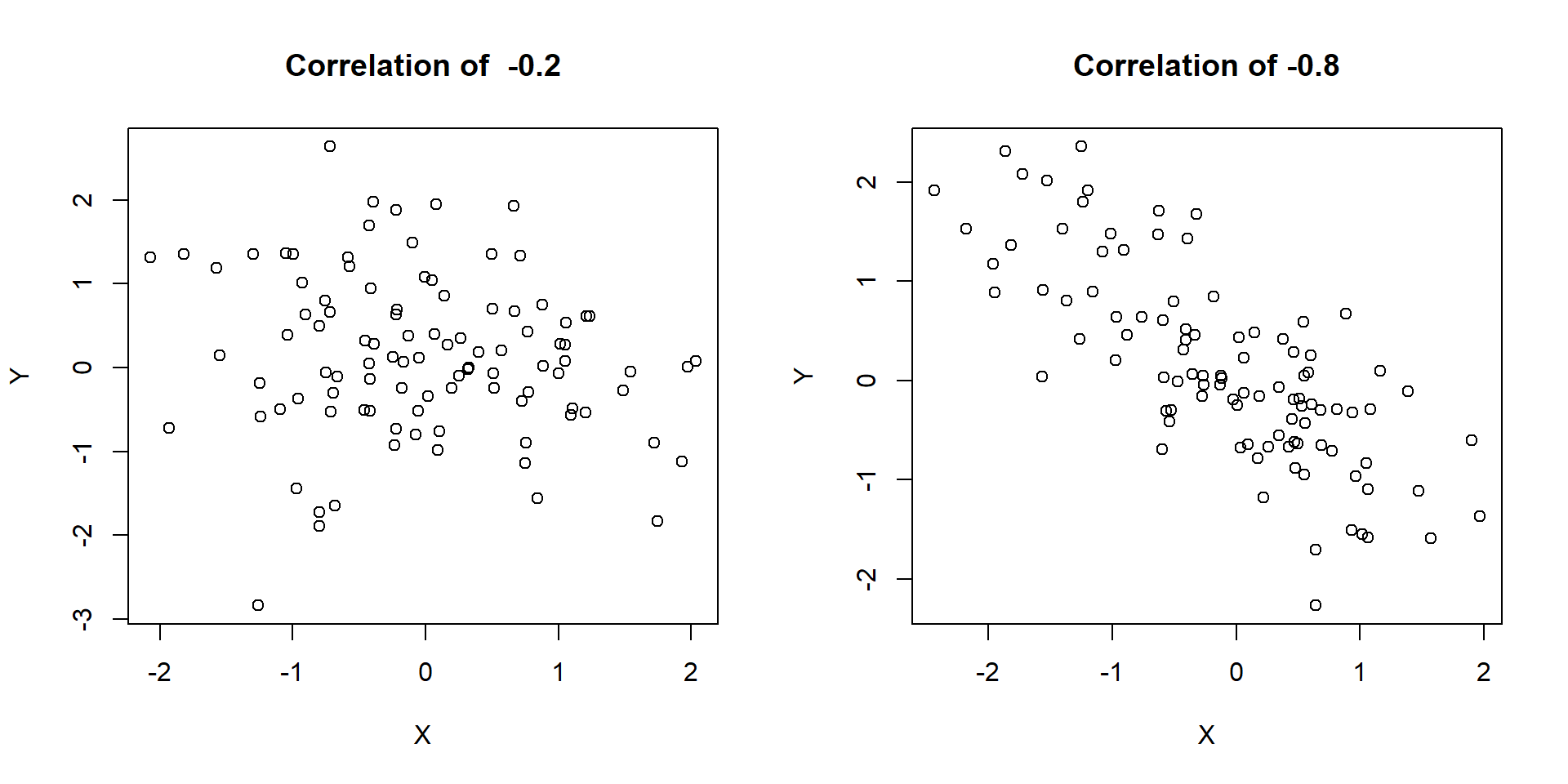
\(\rho < 0\) implies negative correlation
\(\rho = 0\) is consistent with no linear relationship between variables (again, this does not imply that no relationship exists!)
What does it mean to have a correlation of -1 or 1?
Visualizing \(\rho\)
Visualizing \(\rho\)
Visualizing \(\rho\)
Pearson’s correlation coefficient
Pearson’s correlation \(r\) gives and estimate of \(\rho\) as follows. Assuming our observed data are the pairs \((x_1, y_1), (x_2, y_2), \ldots, (x_n, y_n)\), we can calculate \(r\) as
\[r = \frac{1}{n} \sum_{i=1}^n \left(\frac{x_i - \bar{X}}{S_x}\right)\left(\frac{y_i - \bar{Y}}{S_y}\right)\]
\[= \frac{\sum_{i=1}^n (x_i - \bar{X})(y_i - \bar{Y})}{\sqrt{\sum_{i=1}^n (x_i - \bar{X})^2\sum_{i=1}^n(y_i - \bar{Y})^2}}\]
No need to memorize this!…we’ll just use the cor() function to calculate it in R.
Anscombe’s quartet
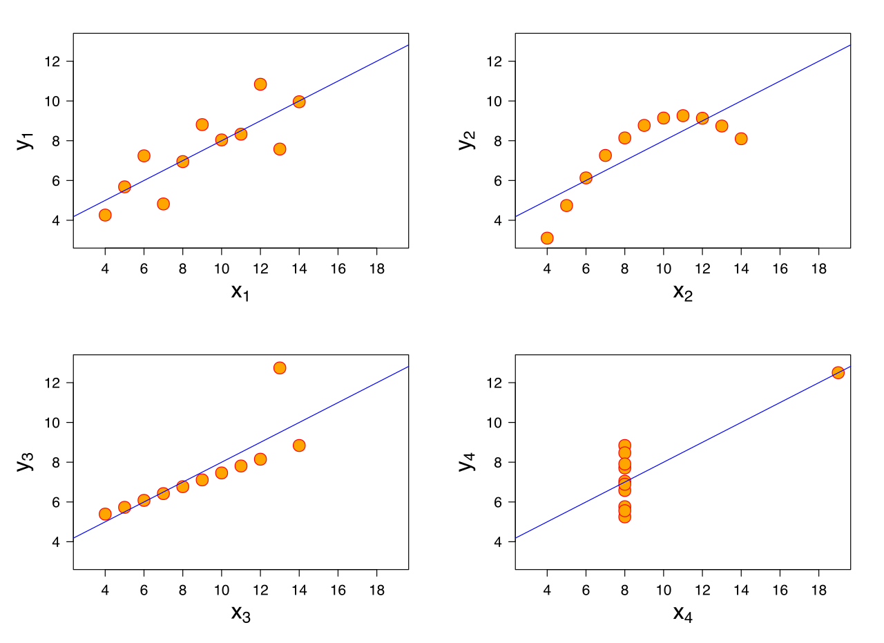
Anscombe’s quartet
In each of the datasets the following statistical summaries hold:
mean of
x: 9variance of
x: 11mean of
y: 7.5variance of
y: 4.125correlation between
xandy: 0.816
Takeaway
Takeaway: Visualizing your data is important! Summary statistics alone cannot capture the full relationship between x and y.
Also, Datasaurus Dozen!
Correlation does not imply causation
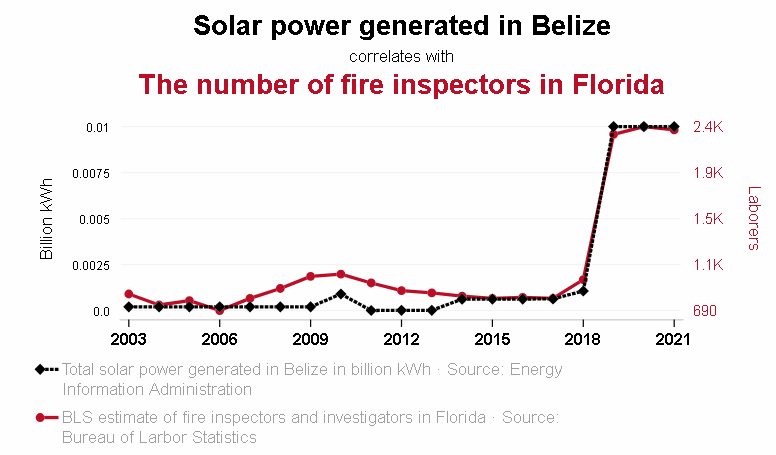
Source: Tyler Vigen, Spurious Correlations
Confounding
Many of these spurious correlations are due to confounding - when a third lurking variable is responsible for the observed relationship.
Example: A near perfect negative correlation (r = -0.99) was seen between cholera mortality and elevation above sea level during a 19th century epidemic.
The observed relationship between cholera and elevation was confounded by a lurking variable, proximity to polluted water.
ggcorrplot
ggcorrplotis a fantastic function for making correlation plots in R.This function is in the
ggcorrplotpackage.
- Let’s check out some examples.
Example
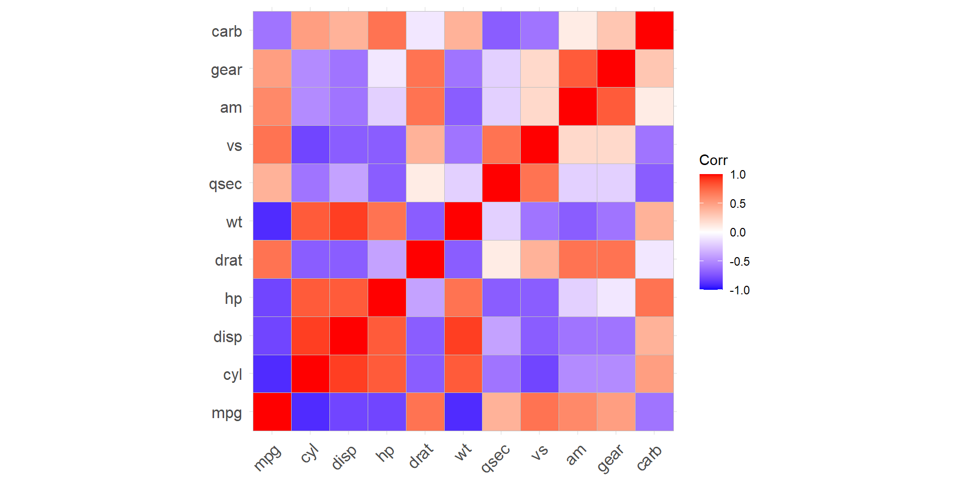
mtcarsis a built-in R dataset, taken from the 1974 Motor Trend US magazine. It has fuel consumption and 10 aspects of automobile design/performance for 32 automobiles.
      mpg  cyl disp   hp drat   wt
mpg   1.0 -0.9 -0.8 -0.8  0.7 -0.9
cyl  -0.9  1.0  0.9  0.8 -0.7  0.8
disp -0.8  0.9  1.0  0.8 -0.7  0.9
hp   -0.8  0.8  0.8  1.0 -0.4  0.7
drat  0.7 -0.7 -0.7 -0.4  1.0 -0.7
wt   -0.9  0.8  0.9  0.7 -0.7  1.0
Plotting the correlation: code
Plotting the correlation: output
Testing the correlation
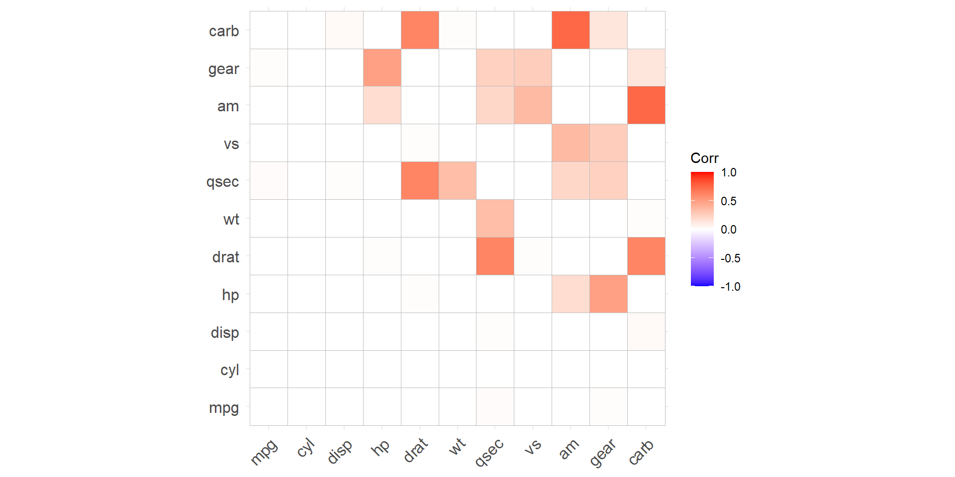
- We can also test whether or not each correlation is statistically equal to zero.
\[H_0: \rho = 0 \quad \text{vs.} \quad H_A: \rho \neq 0\]
              mpg          cyl         disp           hp
mpg  0.000000e+00 6.112687e-10 9.380327e-10 1.787835e-07
cyl  6.112687e-10 0.000000e+00 1.802838e-12 3.477861e-09
disp 9.380327e-10 1.802838e-12 0.000000e+00 7.142679e-08
hp   1.787835e-07 3.477861e-09 7.142679e-08 0.000000e+00
drat 1.776240e-05 8.244636e-06 5.282022e-06 9.988772e-03
wt   1.293959e-10 1.217567e-07 1.222320e-11 4.145827e-05
Example: code
R Graph Gallery
R Graph Gallery has lots of examples, with code!
- Along with many other types of plots.
Application Exercise: taking a closer look at mtcars
On course website.
Next class
- Review for Exam 02