Lecture 17: Introduction to linear regression

BIOS 600 - Spring 2026

Announcements

HW 7 will be assigned Thursday.
Lab 7 will be due Friday.

Reading

P&G Chapter 18
OI: Chapter 8

Back to Lab 2…

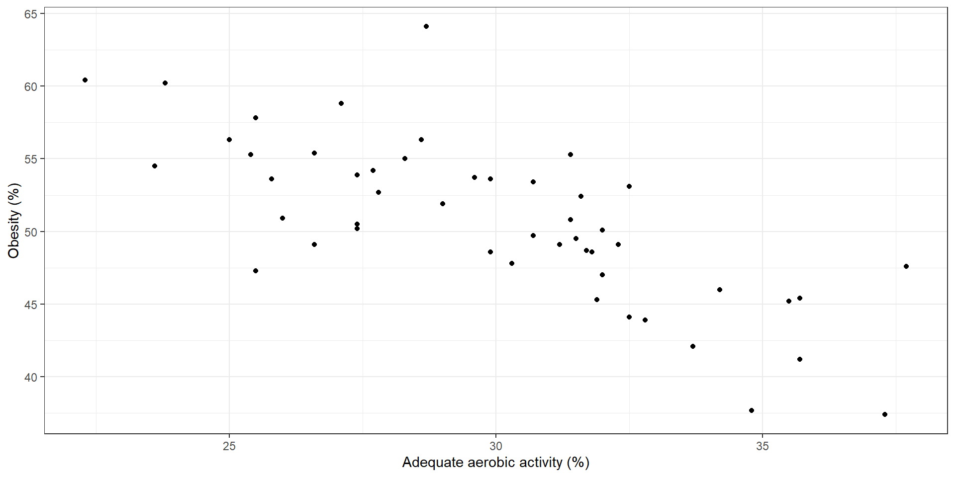
Correlation and regression

Correlation measures the direction and strength of linear relationships
Regression can be used to further quantify these relationships
A regression line summarizes the relationship between explanatory or predictor variables (e.g., Exercise % or \(X\)) and response or outcome variables (e.g., Obesity % or \(Y\))
The fitted regression line can be used to predict the outcome for a given set of predictor values. Our predictions do have error, called residuals (vertical distance between observation and the regression line).
The least-squares regression line minimizes the sum of the squared errors.

Regression

In regression, we use one variable (or more) to try to predict values of another.
In simple linear regression, one variable \(Y\) is the response or outcome or dependent variable and the other \(X\) is the predictor or explanatory variable or independent variable.
This distinction is critical. The regression of \(Y\) on \(X\) is not equal to the regression of \(X\) on \(Y\)
The regression of \(Y\) on \(X\) can be used to predict \(Y\) based on fixed values of \(X\).

Back to Lab 2…

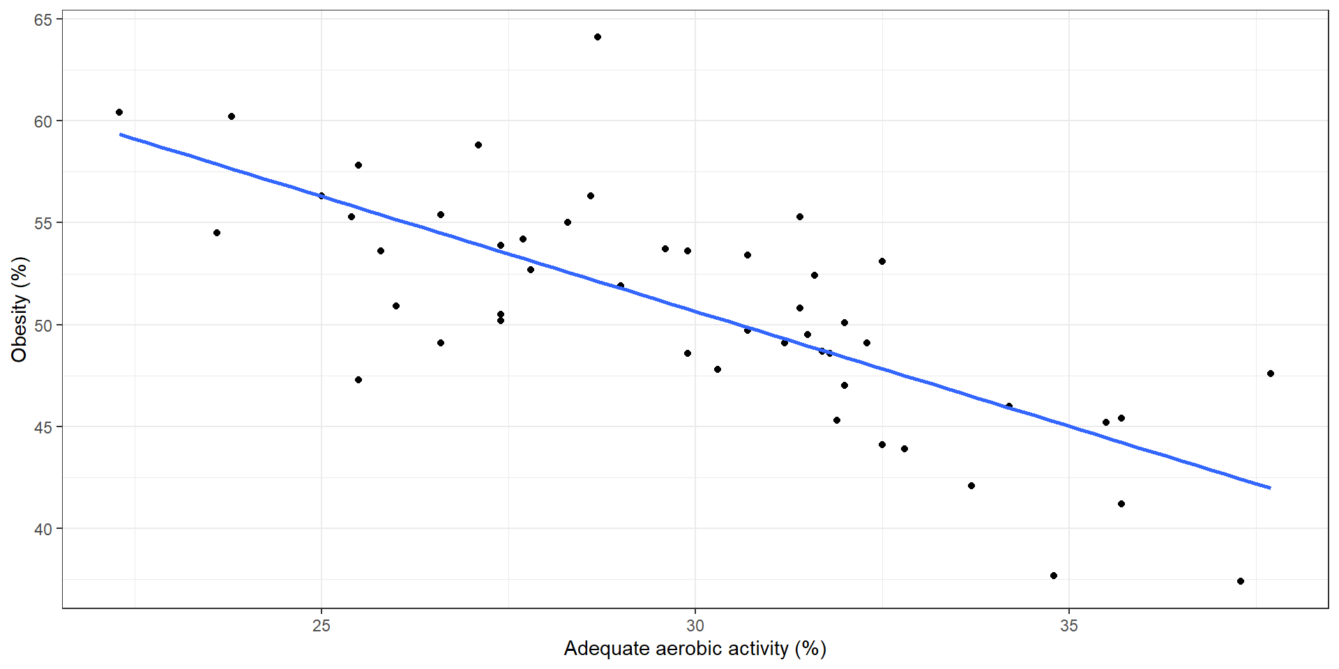
We see the regression line relating exercise and obesity %
Points represent actual data values; note that the line is not a perfect fit

Code for previous slide

cdc |>
  ggplot(aes(x = Obesity, y = Exercise)) +
  geom_point() +
  theme_bw() +
  labs(x = "Adequate aerobic activity (%)", 
       y = "Obesity (%)") +
  geom_smooth(method = "lm", se = F)

The linear model

The model is given by \(y_i=β_0+β_1x_i+ϵ_i\), where

\(y_i\) is the outcome (dependent variable) of interest
\(\beta_0\) is the intercept parameter
\(\beta_1\) is the slope parameter
\(x_i\) is the predictor variable
\(\epsilon_i\) is the error (like \(\beta_0\) and \(\beta_1\), it is not observed)

The \(i\) is an index of observations. So, each observation of the outcome is related to an observation of that individual’s value of the predictor.

The least squares model

Fitted line equation:

\[\hat y_i = \hat \beta_0 +\hat \beta_1 x_i\]

Residual:

\[\hat \epsilon_i = y_i - (\hat \beta_0 +\hat \beta_1 x_i) = y_i - \hat y_i\]

Least squares selects \(\hat β_0\) and \(\hat β_1\) such that the error sum of squares

\[\sum_{i=1}^n \hat \epsilon_i^2 = \sum_{i=1}^n (y_i - \hat y_i)^2\]

is minimized.

Review slope-intercept form of a line

Recall the slope-intercept form of a line, \(y=mx+b\).

\(b\) is the y-intercept, or where the line crosses the y-axis. It is the predicted value of \(y\) when \(x = 0\)
\(m\) is the slope, which tells us the predicted increase in \(y\) when \(x\) changes by 1 unit

Review: formula of a line

Review

Consider the line \(y=3x+1\).

What value does \(y\) take when \(x=0\)?
As \(x\) increases by 1 unit, how much do we expect \(y\) to increase by?

In statistics, we often represent the slope with \(β_1\) and the intercept with \(β_0\), and these values are usually not known but must be estimated.

Model output

fit <- lm(Obesity ~ Exercise, data = cdc)
summary(fit)


Call:
lm(formula = Obesity ~ Exercise, data = cdc)

Residuals:
   Min     1Q Median     3Q    Max 
-6.118 -1.150 -0.065  1.385  6.229 

Coefficients:
            Estimate Std. Error t value Pr(>|t|)    
(Intercept) 54.79087    3.24772  16.871  < 2e-16 ***
Exercise    -0.48991    0.06365  -7.697 6.34e-10 ***
---
Signif. codes:  0 '***' 0.001 '**' 0.01 '*' 0.05 '.' 0.1 ' ' 1

Residual standard error: 2.455 on 48 degrees of freedom
Multiple R-squared:  0.5524,    Adjusted R-squared:  0.5431 
F-statistic: 59.25 on 1 and 48 DF,  p-value: 6.336e-10

A neater way

library(tidymodels)
library(kableExtra)

tidy(fit) |>
  kable()

term	estimate	std.error	statistic	p.value
(Intercept)	54.7908720	3.2477165	16.870583	0
Exercise	-0.4899056	0.0636478	-7.697129	0

Can we do better?

Even better

tidy(fit) |>
  kable(digits = 3) # round to 3 digits

term	estimate	std.error	statistic	p.value
(Intercept)	54.791	3.248	16.871	0
Exercise	-0.490	0.064	-7.697	0

Note: p-values are not actually 0. They are just quite small so they get rounded to zero in the table.

Tip

In your homework, display the output with tidy() and kable() like this!

Intercept and slope

The intercept is the estimated mean outcome when the predictor is zero (does this make sense in context?)
The slope is the expected change in the outcome corresponding to a one-unit change in the predictor

Slope Interpretation: For each percentage increase in Exercise, we expect the Obesity percentage to decrease by .48.

Tip

For all interpretations, remember to include units!

Intercept interpretation

When zero percent of the region’s population gets adequate Exercise, we would expect the percent of the region that is obese to be 54.79%.
Does it make sense to interpret the intercept here?
You should only interpret the intercept in a regression model if:
- the predictor can feasibly take values equal to or near zero, or
- there are values near zero in the observed data

Let’s check

hist(cdc$Exercise)

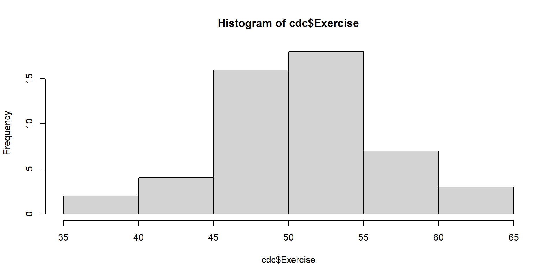
Let’s check

min(cdc$Exercise)

[1] 37.4

Since the predictor (Exercise) does not feasibly take on values equal to zero (and we also checked that the lowest value in the dataset is 37.4%), we should not interpret the intercept.

Model assumptions

Assumptions of the model \(y_i = \beta_0 + \beta_1 x_1 + \epsilon_i\) include:

The outcomes \(y_i\) are independent. This is violated if our study contains repeated outcome measures on an individual, if siblings are enrolled, etc.
A linear relationship holds (though we can relax this to some extent)
For a specified value of \(x\), which is measured without error, \(y_i∼N(β_0+β_1x_i,σ^2)\). Note that this implies \(ϵ_i∼N(0,σ^2)\).
The variance \(σ^2\) is constant across all values of \(x\); this is called homogeneity of variance

Hypothesis testing

The primary hypothesis test of interest is usually \(H_0:β_1=0\) (There is no association between exercise and obesity percentage) versus \(H_1:β_1≠0\) (there is an association between exercise and obesity percentage.)
Under the null hypothesis, we can use a t-test to test this.
R automatically tests this with the lm() function, and provides the t-statistic and p-value in the output.

term	estimate	std.error	statistic	p.value
(Intercept)	54.791	3.248	16.871	0
Exercise	-0.490	0.064	-7.697	0

Given our t-statistic of -7.7 and p-value of <0.001, what might we conclude in our data?

Some additional output

summary(fit)$r.squared

[1] 0.55243

The \(R-squared\) value indicates that exercise explains 55% of the variance of obesity.
\(R^2\) tells us about how much of the variability in obesity is explained by exercise; as it gets close to 1, the points get tighter around the regression line.
“Variance explained” does not mean we think a causal relationship exists!

Predicted values

The regression equation can be used to get predicted means at any value of \(x\).
\(\hat y_i=\hat β_0+ \hat β_1x_i\), where we call \(\hat y\) the predicted value of \(y\) at a given value of \(x\) (what happened to the error term?).

Predicted values

For the CDC data that predicts a state’s obesity percentage by its adequate exercise percentage, we have

\[\hat y_i = 54.79 - 0.49 x_i\]

So, the predicted mean obesity percentage for a state where 50% of residents get adequate exercise is

\[\hat y_i = 54.79 - 0.49 (50) \]

We would predict an obesity percentage of approximately 30%. Note the importance of getting the units correct.

Application exercise

For the remaining time, start on AE 6 on the course website
Due Thursday of next week

Recap

What is a linear regression model? How do we fit & visualize the model in R?
Slope, intercept and interpretations
Understand when it’s appropriate to interpret the intercept
Interpret \(R^2\) from regression output

Next class

We will learn how to check the regression model assumptions in R
Multiple regression