Lecture 18: Multiple Linear Regression
BIOS 600 - Spring 2026
Announcements
Lab 7 due Friday April 10
HW 7 canceled, will provide some extra exam prep materials early
Reading
P&G: Chapter 19
OI: 9.1 and 9.3
Computational setup
Review: Assumptions of linear regression
Review
Independent observations
Linear relationship between predictor and response
Conditional on predictor(s), the response follows a normal distribution (normally distributed residuals)
Equal variances (homogeneity of variance in the residuals)
How can we check the assumptions to ensure they are met?
We can do so by “running regression diagnostics” - checking the assumptions within our regression model.
Regression diagnostics: independence
We just have to think through this one, unfortunately.
The independence assumption means that each observation provides unique information — no observation should influence another.
In other words, the residuals (errors) should not be correlated with each other.
Common violations of independence
Repeated measurements on the same subject over time
(e.g., daily blood pressure readings for the same patient)Clustered or grouped data
(e.g., patients within the same hospital, students within a classroom)Time-series data
(e.g., monthly pollution levels, daily step counts)
Regression diagnostics: equal variance; linearity
To check equal variances and linearity, we can use a plot of the residuals \(\hat ϵ_i\) by the predicted (or fitted) values \(\hat y_i\).
We expect to see evenly-spaced dots along the y axis (equal variances), with symmetrically distributed observations around the y axis (linearity). Patterns or trends are evidence something is wrong. (Drawing on board.)
Regression diagnostics: equal variances
- Usually plot residuals against fitted values, and look for patterns in the spread of residuals.
Regression diagnostics: normality of errors
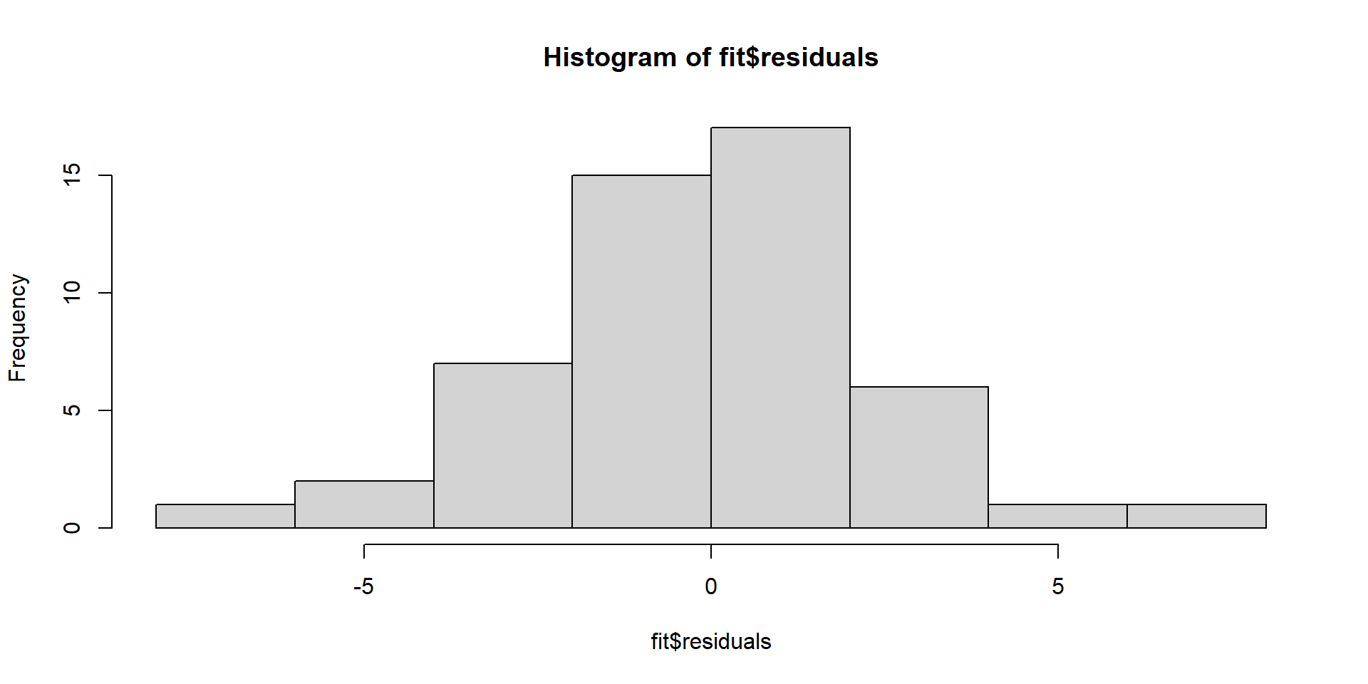
- Use a histogram of the residuals to check normality. There are more advanced methods and plots, but we won’t talk about them here
Checking assumptions for our model…
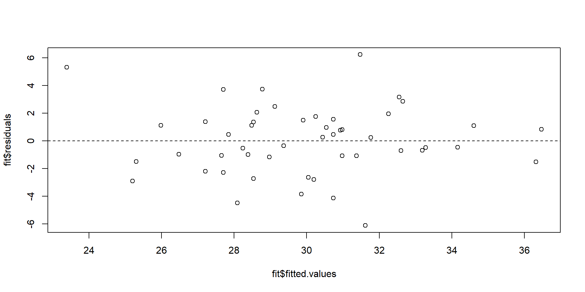
Checking assumptions for our model…
Back to Lab 02
In Lab 2 we examined the regression of obesity percentage on adequate exercise percentage.
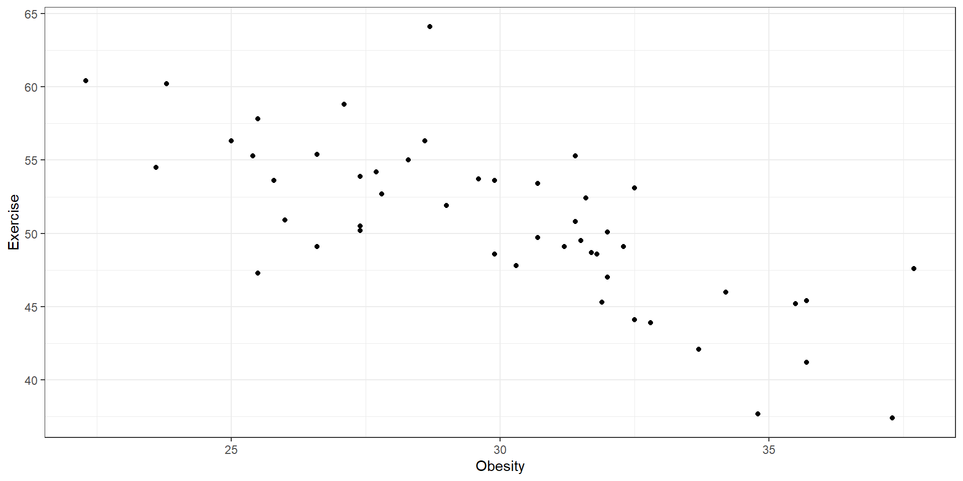
Do we think this is the only factor that can help us predict obesity percentage?
Multiple regression
The multiple regression model extends the simple linear regression model by incorporating more than one explanatory variable.
The assumptions are similar to those of the simple linear regression model. This type of model is often called a multivariable (not multivariate) model.
Multiple regression is often used to control for confounders or predictors that explain variability in the response:
Knowing a state has above average exercise percentage might tell you something about the obesity percentage
If you also knew that state’s HDI category, you might be able to do even better!
Multiple regression
Importantly, accounting for multiple predictors allows us to address potential confounding.
We are looking at relationships while holding others constant - for instance, we know that exercise percentage and HDI category might be correlated. Perhaps any associations between obesity and exercise percentage we see are actually driven by HDI category.
Multiple regression
By fitting a multiple linear regression model, we can look at associations between obesity and exercise percentage while holding HDI constant (that is, at each possible value of HDI, what is the “remaining relationship” between exercise and obesity percentage?).
Similarly, we can also look at associations between HDI and obesity while holding exercise constant (that is, at each possible value of exercise %, what is the “remaining relationship” between HDI and obesity percentage?).
Multiple regression
The model is given by
\[y_i = \beta_0 + \beta_1 x_{1i} + \beta_2 x_{2i} + \cdots + \beta_p x_{pi} + \epsilon_i\]
\(p\) is the total number of predictor or explanatory variables
\(y_i\) is the outcome (dependent variable) of interest
\(\beta_0\) is the intercept parameter
\(\beta_1, \beta_2, \cdots, \beta_p\) are the slope parameters
\(x_{1i}, x_{2i}, \cdots, x_{pi}\) are predictor variables
\(\epsilon_i\) is the error (like the \(\beta\)s, it is not observed)
Assumptions are essentially the same as in simple linear regression.
Multiple regression
Consider the model
\[Obesity_i = \beta_0 + \beta_1 Exercise_i + \beta_2 Smoking_i + \epsilon_i\]
Parameter Meaning
What might the parameters \(\beta_0\), \(\beta_1\), and \(\beta_2\) represent?
Multiple regression
Call:
lm(formula = Obesity ~ Exercise + Smoking, data = cdc)

Residuals:
    Min      1Q  Median      3Q     Max
-3.6884 -1.4006  0.1385  1.3435  3.6176

Coefficients:
            Estimate Std. Error t value Pr(>|t|)
(Intercept) 36.10015    3.86311   9.345 2.72e-12 ***
Exercise    -0.30899    0.05579  -5.538 1.34e-06 ***
Smoking      0.54249    0.08716   6.224 1.23e-07 ***
---
Signif. codes:  0 '***' 0.001 '**' 0.01 '*' 0.05 '.' 0.1 ' ' 1

Residual standard error: 1.837 on 47 degrees of freedom
Multiple R-squared:  0.7546,    Adjusted R-squared:  0.7442
F-statistic: 72.28 on 2 and 47 DF,  p-value: 4.572e-15
Multiple regression: kable
| term | estimate | std.error | statistic | p.value |
|---|---|---|---|---|
| (Intercept) | 36.100 | 3.863 | 9.345 | 0 |
| Exercise | -0.309 | 0.056 | -5.538 | 0 |
| Smoking | 0.542 | 0.087 | 6.224 | 0 |
How might we interpret these parameter estimates? (watch out for the scale!)
Interpretation
- Interpreting \(\hat{\beta_1}\): For every one percent increase of adults who participated in at least 2.5 hours of aerobic activity per week, we expect the percent of adults who are obese to decrease by .308 of a percentage point on average, holding Smoking constant.
Your turn
Use the interpretation above to write out an interpretation of \(\hat{\beta_2}\). Recall that the Smoking variable is defined as percent of adults in region who smoked at least one cigarette in the past month.
Hypotheses of interest
Hypotheses of interest may include hypotheses for single parameters:
- For instance, \(H_0:β_1=0\) vs. \(H_1:β_1≠0\). In our previous model, this would test whether there is a linear association between exercise % and obesity %, while controlling for smoking %
This is tested using a t-test with \(n−k\) degrees of freedom, where \(n\) is the number of observations in the model and \(k\) is the number of estimated model parameters (including the intercept and all slope terms, but not including the error variance).
Hypotheses of interest
Say we were to test this hypothesis for our model. What might we conclude?
| term | estimate | std.error | statistic | p.value |
|---|---|---|---|---|
| (Intercept) | 36.100 | 3.863 | 9.345 | 0 |
| Exercise | -0.309 | 0.056 | -5.538 | 0 |
| Smoking | 0.542 | 0.087 | 6.224 | 0 |
In this case, the p-value was lower than the pre-specified significance cut-off. There is sufficient evidence to suggest that, controlling for smoking %, there is a non-zero linear association between exercise % and obesity % by state.
Hypotheses of interest
We might also test multiple parameters at once (for instance, all the slopes):
- \(H_0: \beta_1 = \beta_2 = 0\) vs. \(H_1:\) at least one of the \(\beta_k\) is not 0. (variable has a linear association with exercise %)
This is given by an F test (much like ANOVA!) with numerator df equal to the number of parameters being tested (here, the number of slopes, i.e. 3) and denominator df equal to \(n−k\) (number of observations minus number of estimated model parameters, including the intercept).
What might we conclude for the overall F test for our model, assuming \(\alpha = 0.05\)?
F-test
This information is given in the original summary(model):
Call:
lm(formula = Obesity ~ Exercise + Smoking, data = cdc)

Residuals:
    Min      1Q  Median      3Q     Max
-3.6884 -1.4006  0.1385  1.3435  3.6176

Coefficients:
            Estimate Std. Error t value Pr(>|t|)
(Intercept) 36.10015    3.86311   9.345 2.72e-12 ***
Exercise    -0.30899    0.05579  -5.538 1.34e-06 ***
Smoking      0.54249    0.08716   6.224 1.23e-07 ***
---
Signif. codes:  0 '***' 0.001 '**' 0.01 '*' 0.05 '.' 0.1 ' ' 1

Residual standard error: 1.837 on 47 degrees of freedom
Multiple R-squared:  0.7546,    Adjusted R-squared:  0.7442
F-statistic: 72.28 on 2 and 47 DF,  p-value: 4.572e-15
Hypotheses of interest
Conclusion: In this case, the p-value (4.572e-15) was lower than the pre-specified significance cut-off. There is sufficient evidence to suggest that at least one predictor (Exercise and/or Smoking) has a non-zero linear association with obesity %.
Multiple Regression in Real Life
Tip
Based on this paper, answer the following questions:
In 1-2 sentences, describe the goal of this study/analysis.
What was the outcome variable?
How many independent variables did they use in their multiple regression model?
In Table 4, what was the F-value and p-value? What is your conclusion?
Which four predictor variables most significantly influenced the outcome?
Confidence intervals
For individual predictors, we can also use the standard error estimate to construct confidence intervals. These intervals are constructed using a critical value from a t distribution:
\[(\hat \beta_k - t^*_{1-\alpha/2; n-k} \times SE(\hat \beta_k), \hat \beta_k + t^*_{1-\alpha/2; n-k} \times SE(\hat \beta_k))\]
For instance, \(SE (\hat \beta_1)=0.06\). Thus, we have that a 95% confidence interval for \(β_1\) is (-0.43, -0.19). If we were to interpret this interval, it would have to be conditionally on the other variables in the model.
R-squared
In our model, \(R^2=0.7546\), suggesting that about 75% of the variability in obesity percentage can be explained by our model.
However, \(R^2\) can never decrease when variables are added to a model, even if they are useless.
Thus, we can use adjusted \(R^2 \leq R^2\), where the adjustment is made to account for the number of predictors.
The adjusted \(R^2\) incorporates a penalty for each additional variable in a model, so that the adjusted \(R^2\) will go down if a new variable does not improve prediction much, and it will go up if the new variable does improve prediction, conditional on the other variables already in the model.
With that said, \(R^2\) or adj. \(R^2\) should never be used as the only reasons to select variables for your model - you must rely on scientific knowledge and context!
Categorical predictors
We often have categorical predictors in modeling settings (for instance, here we have HDI). However, it might not make sense to think about a “one unit increase” in a categorical variable (how would that even work?)
In regression settings, we can account for categorical variables by creating dummy variables, which are indicator variables for certain conditions happening. For instance, there are three categories of HDI in the dataset: bottom ten, middle, and top ten.
When considering categorical variables, one variable is taken to be the baseline or reference value. All other categories will be compared to it.
Categorical predictors
Suppose the “top ten” category is taken to be the referent value. Then we can create two dummy variables:
HDI == Middle: 1 if this condition is true; 0 otherwise
HDI == Bottom Ten: 1 if this condition is true; 0 otherwise
Interpretation of dummy variables
Consider the model
\[Obesity_i = \beta_0 + \beta_1(HDI == Middle)_i + \]
\[ \beta_2(HDI == BottomTen)_i + \epsilon_i\]
The parameter interpretations are below.
\(\beta_0\) represents the expected obesity percentage for a state with 0 for the two dummy variables. That is, in the top ten HDI
\(\beta_1\) represents the expected difference in obesity percentage for a state in the middle HDI category, compared to the top ten
\(\beta_2\) represents the expected difference in obesity percentage for a state in the bottom ten HDI category, compared to the top ten
Note that we had to estimate multiple “slopes” for this one variable - one corresponding to each non-reference level.
Interpretation of dummy variables
| term | estimate | std.error | statistic | p.value |
|---|---|---|---|---|
| (Intercept) | 34.430 | 0.816 | 42.195 | 0 |
| HDIMiddle | -4.797 | 0.942 | -5.091 | 0 |
| HDITop ten | -8.080 | 1.154 | -7.002 | 0 |
How would you interpret the estimates?
Changing the reference level
- Wait a minute! R automatically assigned the lowest level of HDI as the reference level. Let’s see how we can change the reference level:
This reorders the factor levels so that “
Top ten” becomes the first (reference) level.Now, when we run the regression, the model will automatically use
Top tenas the baseline.
Re-running the model
| term | estimate | std.error | statistic | p.value |
|---|---|---|---|---|
| (Intercept) | 26.350 | 0.816 | 32.293 | 0.000 |
| HDI_relevelBottom ten | 8.080 | 1.154 | 7.002 | 0.000 |
| HDI_relevelMiddle | 3.283 | 0.942 | 3.485 | 0.001 |
Interpretation of dummy variables
| term | estimate | std.error | statistic | p.value |
|---|---|---|---|---|
| (Intercept) | 44.897 | 3.406 | 13.184 | 0.000 |
| Exercise | -0.348 | 0.063 | -5.545 | 0.000 |
| HDI_relevelBottom ten | 5.125 | 1.049 | 4.887 | 0.000 |
| HDI_relevelMiddle | 2.753 | 0.744 | 3.702 | 0.001 |
How would you interpret these estimates?
Recap
How to check regression diagnostics
How to interpret model coefficients in a multiple regression model
Interpreting results of an overall F-test in a multiple regression model
Adjusted \(R^2\) vs. \(R^2\)
Interpreting coefficient estimates for categorical predictors
Next time
Interactions, collinearity
Logistic regression (if time)