Lecture 20: Logistic regression
BIOS 600 - Spring 2026
Announcements
- Final exam May 5, 8am, this room
- Please let me know ASAP if you need to reschedule (and have a valid reason)
Overview
Computational setup
Very optional reading
P&G Chapter 20
OI: Section 9.5
Multicollinearity
One common problem in multiple regression is multicollinearity, which occurs when multiple highly correlated variables are used as predictors.
Collinearity simply refers to two variables behind highly correlated.
In this case, the model can become unstable (often seen as standard errors that get huge and lead to huge confidence interval estimates), and it can be difficult to assess the relationships of the predictors.
Diagnosing multicollinearity
If nothing is significant when you “expect” something to be, we have some clues:
Individual predictors are significant in simple linear regression models,
but standard errors and interval estimates are huge,
and the overall F test is significant
A significant overall F test with no significant individual variable test is a typical sign of collinearity. We can check out the correlations among the three predictors.
Checking VIF
Another way to check for multicollinearity is through VIF values. VIF values indicate the extent of multicollinearity.
VIF values could range from 1 to infinity.
A VIF value of 1 suggests no correlation with other predictors.
Values between 1 and 5 generally indicate moderate correlation.
Values above 5 (or sometimes 10, depending on the context) are often considered problematic, indicating severe multicollinearity and potential issues with coefficient stability and interpretation.
VIF
- Let’s say we had the following model:
Exercise  Smoking   Over65
1.420894 1.541720 1.123272 - In this model, none of the VIFs are above 5 (in fact, they’re much closer to 1), so multicollinearity is not an issue here.
Logistic regression
Models for binary outcomes
- Suppose we have a binary outcome variable (e.g., \(Y = 1\) if a condition is satisfied and 0 otherwise), and potentially multiple predictors on a variety of scales.
What distribution does our outcome have?
Models for binary outcomes
- Suppose we want to model \(P(Y=1)\), the success probability. One strategy might be to simply fit a linear regression model to the probabilities:
\[P(Y_i = 1) = \beta_0 + \beta_1 x_{i1} + \cdots + \beta_p x_{ip} + \epsilon_i\]
Is this a reasonable approach? Why or why not?
Primary biliary cirrhosis
The Mayo Clinic conducted a trial for primary biliary cirrhosis, comparing the drug D-penicillamine vs. placebo. Patients were followed for a specified duration, and their status at the end of follow-up (whether they died) was recorded. Researchers are interested in predicting whether a patient died based on the following variables:
ascites: whether the patient had ascites (abnormal fluid buildup in the abdomen) (1 = yes, 0 = no)bili: serum bilirubin in mg/dL (higher values may indicate liver damage/disease)stage: histologic stage of disease (ordinal categorical variable with stages 1, 2, 3, and 4)
What can go wrong?
Suppose we fit the following model:
\[P(Y_i = 1) = \beta_0 + \beta_1 asc_i + \beta_2 bili_i + \beta_3 s2_i + \beta_4 s3_i + \beta_5 s4_i + \epsilon_i\]
where \(Y=1\) if a patient died during the study follow-up.
What can go wrong?
What could go wrong?
- We can technically fit the model:
| term | estimate | std.error | statistic | p.value |
|---|---|---|---|---|
| (Intercept) | 0.025 | 0.107 | 0.235 | 0.815 |
| ascites | 0.283 | 0.102 | 2.786 | 0.006 |
| bili | 0.035 | 0.006 | 5.938 | 0.000 |
| as.factor(stage)2 | 0.131 | 0.119 | 1.103 | 0.271 |
| as.factor(stage)3 | 0.230 | 0.114 | 2.015 | 0.045 |
| as.factor(stage)4 | 0.355 | 0.117 | 3.037 | 0.003 |
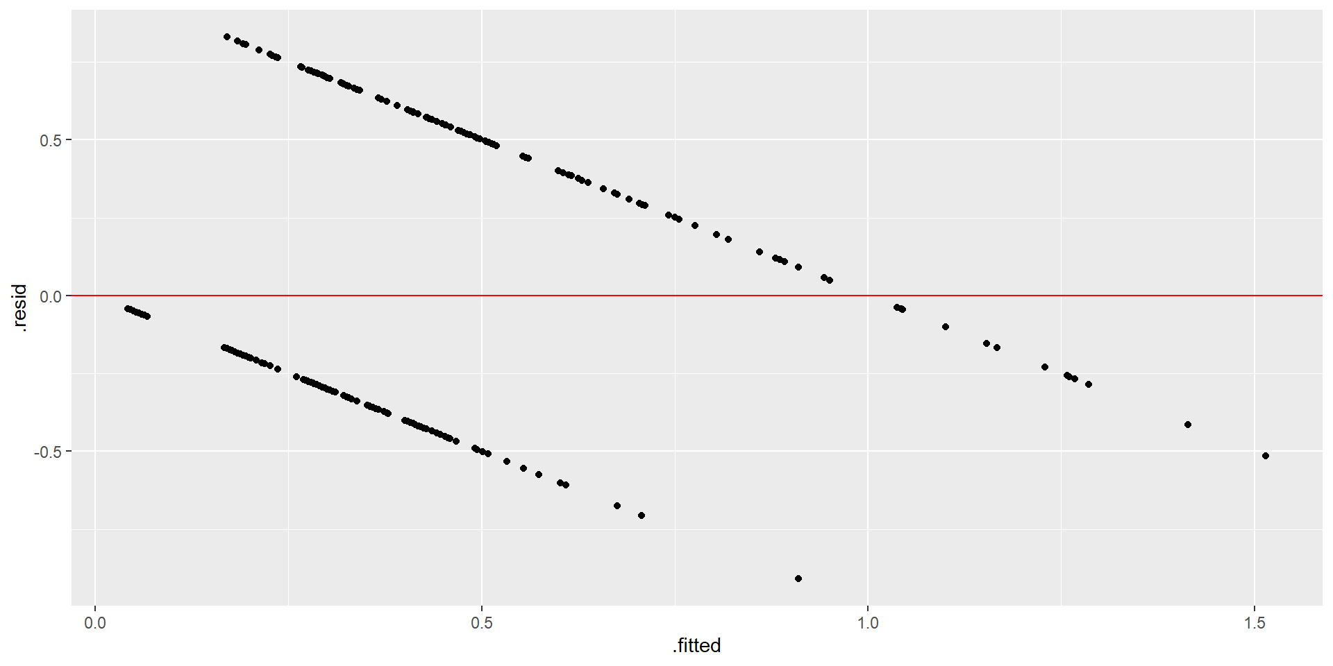
- However, let’s check the fitted vs. residuals plot.
What could go wrong?
From probabilities to log odds
Suppose the probability of an event is \(p\).
Then the odds that the event occurs is \(\frac{p}{1-p}\)
Taking the natural log of the odds, we have the logit of \(p\) (also known as the log-odds):
\[logit(p) = \text{log} \left(\frac{p}{1-p}\right)\]
- Although \(p\) is constrained to lie between 0 and 1, the logit of \(p\) can be anything from \(-\infty\) to \(\infty\).
Logistic regression model
Let’s create a linear model for the log-odds:
\[logit(p_i) = \text{log} \left(\frac{p_i}{1-p_i}\right) = \beta_0 + \beta_1 x_{i1} + \cdots + \beta_p x_{ip}\]
This is the logistic regression model.
In this model, it’s ok that we could get any potential value for the logit of \(p\) (can range from \(-\infty\) to \(+ \infty\).
We can always back-transform a prediction to be a valid probability between 0 and 1.
Logistic regression model
\[logit(p_i) = \text{log} \left(\frac{p_i}{1-p_i}\right) = \beta_0 + \beta_1 x_{i1} + \cdots + \beta_p x_{ip}\]
Negative logits represent probabilities less than one-half.
Positive logits represent probabilities above one-half.
Interpreting parameters
Typically we interpret functions of parameters in logistic regression rather than the parameters themselves. For the simple model
\[\text{log} \left(\frac{p_i}{1-p_i}\right) = \beta_0 + \beta_1 x_{i}\]
then the probability that \(Y = 1\) when \(X = 0\) is
\(\frac{\text{exp}(\beta_0)}{1 + \text{exp}(\beta_0)}\)
- How did we get this?
Warning
Prepare for math ahead!
Solving logistic model for \(p_i\)
\[\text{log} \left(\frac{p_i}{1-p_i}\right) = \beta_0 + \beta_1 x_{i}\]
Interpreting parameters
Suppose that X is a binary (0/1) variable (e.g., X = 1 for smoker and 0 for non-smoker). In this case, we interpret \(\text{exp}(\beta_1)\) as the odds ratio (OR) of the response for the two possible levels of X.
The odds ratio of an event A, for a second event B, is $ $
For X on a continuous scale, \(\text{exp}(\beta_1)\) is interpreted as the odds ratio of the response comparing two values of X one unit apart.
Back to PBC
| term | estimate | std.error | statistic | p.value |
|---|---|---|---|---|
| (Intercept) | -3.143 | 1.054 | -2.981 | 0.003 |
| ascites | 2.868 | 1.067 | 2.689 | 0.007 |
| bili | 0.315 | 0.064 | 4.886 | 0.000 |
| as.factor(stage)2 | 1.251 | 1.095 | 1.142 | 0.253 |
| as.factor(stage)3 | 1.716 | 1.069 | 1.604 | 0.109 |
| as.factor(stage)4 | 2.167 | 1.075 | 2.015 | 0.044 |
Interpretations
\(\hat\beta_{\text{ascites}}\): The estimate for ascites was 2.87. Thus, the odds ratio for dying is exp(2.87), or approx. 17.6. Patients with ascites have 17.6 times the odds of dying compared to patients that do not, holding all other variables constant.
\(\hat\beta_{\text{bili}}\): The estimate for bilirubin was 0.31. Thus, the odds ratio for dying for a patient with 1 additional mg/dL serum bilirubin compared to another is exp(0.31) \(\approx\) 1.36, holding all other variables constant.
\(\hat\beta_{\text{stage 3}}\): The baseline stage was 1. The estimate corresponding to stage 3 was 1.72. Thus, patients in stage 3 have approximately 5.58 times the odds of dying compared to patients with the baseline stage, holding all other variables constant.
Interpreting parameters
Why is this the interpretation for continuous variables?
The log odds of response for X = 1 is given by \(β_0+β_1\), and the log odds of response for X = 0 is \(β_0\).
So the odds ratio of response comparing X = 1 to X = 0 is given by:
\[\frac{\text{exp}(\beta_0 + \beta_1)}{\text{exp}(\beta_0)} = \text{exp}(\beta_1)\]
- In a multiple logistic regression model, this has to be interpreted conditionally on values of other variables in the model (i.e., controlling for them).
Back to PBC
Remember, we are interested in the probability that a patient died during follow-up (a “success”). We are predicting the log-odds of this event happening.
On your own
What are the odds of death for a patient with Stage 4 disease relative to Stage 1, holding all other variables constant?
Predicted probabilities
There is a one-to-one-relationship between \(p\) and \(logit(p)\). So, if we predict the log-odds, we can back-transform to get back to a predicted probability.
For instance, suppose a patient does not have ascites, has a bilirubin level of 5 mg/dL, and is a stage 2 patient. Their predicted log-odds are:
\[−3.14+0.31×5+1.25=−0.34\]
Thus, their predicted probability of dying is
\[\frac{\text{exp}(-0.34)}{1+\text{exp}(-0.34)} = 0.42\]
How did we derive this calculation?
On your own
What is the predicted probability of dying for a patient with ascites, a bilirubin level of 3 mg/dL, and stage 3?
Hypothesis tests in logistic regression
Generally, we wish to know whether the OR = 1 or equivalently, whether the logit of \(p\) (a \(\beta\) coefficient) = 0. To test
\[H_0: \beta_k = 0\]
\[H_1: \beta_k \neq 0\]
we can compare the ratio of a parameter estimate to its standard error using the standard normal distribution (reason we use Z instead of t is a bit technical).
Confidence intervals
CIs for associations on the logit scale are given by
\[\hat \beta_j \pm z^*_{1-\alpha/2} \times \widehat {SE} (\hat\beta_j)\]
These are typically translated into confidence intervals in odds scale by exponentiating the lower and upper limits.