dpois(x = 0, lambda = 1.5)[1] 0.2231302BIOS 600 - Spring 2026
HW 2 due tonight at 11:59pm
Application Exercise due tomorrow (Friday) at 11:59pm
HW 3 (short) will be released after class, due next Thursday at 11:59pm.
Topics list and Formula sheet have been added to the course website.
Lab 4 will be next week, but not on exam. Feel free to use lab time to ask about lab or as TA office hours before the exam on Tuesday 2/17.
If you have any questions, feel free to make a “New Post” on Ed Discussion about it! We are happy to answer any questions, no matter how small.
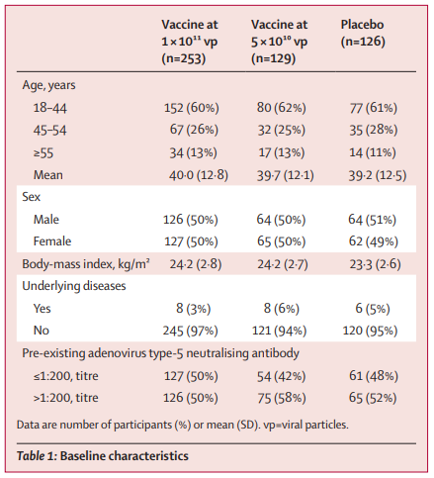
What is the probability that a randomly selected patient in the trial was not assigned to high dose vaccine and had no underlying diseases? Should be: (245 + 120)/508 = 0.718.
Review discrete probability distributions
Poisson distribution
Work on Application Exercise from last time
Expectation and variance
Continuous distributions and examples
There are three rules for discrete probability distributions:
Outcomes must be disjoint
The probability of each outcome must be \(\geq\) 0 and \(\leq\) 1
The sum of the outcome probabilities must add up to 1
| Event | Probability |
|---|---|
| X = pre | 0.10 |
| X = early | 0.27 |
| X = full | 0.57 |
| X = late/post | 0.06 |
Two possible outcomes: “success” (value 1), or “failure” (value 0).
Success occurs with probability p.
E.g.: flipping a fair coin. p=0.5.
Extends the Bernoulli distribution to multiple trials
The number of successes across n independent Bernoulli trials, each with same p.
E.g.: number of heads in five flips of a fair coin.
\[P(X=k) = {n \choose k}p^k (1-p)^{n-k}\]
Discrete distribution taking on possible values 0, 1, 2, \(\ldots\), \(\infty\)
Often used to model counts or rare events
Much like the binomial distribution, requires a few assumptions
The Poisson distribution gives the probability that \(k\) events occur in a given “interval”. There are four assumptions:
Within any interval, \(k\) may take on values 0, 1, 2, 3, \(\ldots\), \(\infty\)
Each event occurs independently, both within the same interval, and between intervals
The average rate at which events occur in an interval, \(\lambda\), is constant
Two events cannot occur simultaneously
What is an “interval”?
If \(X\) has a Poisson distribution, then
\[P(X=k) = \frac{\lambda^k e^{-\lambda}}{k!}\]
What do these components mean?
This expression will always be provided to you if needed.
Suppose on average, there are 1.5 deaths due to Alzheimer’s Disease in a town each year. For a one-year period in this town, what is the chance that two or more people die from Alzheimer’s?
Within any interval, the number of AD deaths can range from 0 to \(\infty\) (technically not true, but close enough)
One individual dying of Alzheimer’s does not affect the chance of another person dying of Alzheimer’s
The AD death rate is constant in this town
Two AD deaths cannot occur at the same time (we can always subdivide time intervals such that only one person experiences this event in a given sub-interval)
Using the formula for a Poisson distribution, write out how you would calculate the probability of zero Alzheimer’s deaths in a year.
Thus \(Z \sim Pois(1.5)\), and \(P(Z=0)\), \(P(Z=1)\), and \(P(Z\geq 2)\) are disjoint events.
So, using the Complement Rule, \(P(Z \geq 2) = 1- [P(Z = 0) + P(Z = 1)]\), where
\[ \begin{aligned} P(Z=0) &= \frac{1.5^0 \times e^{-1.5}}{0!}\approx 0.223 \\ P(Z=1) &= \frac{1.5^1 \times e^{-1.5}}{1!}\approx 0.335 \end{aligned} \]
And so \(P(Z \geq 2) \approx 1-0.223-0.335 = 0.442\).
We can calculate these values in R using the dpois() function:
dpois(x = 0, lambda = 1.5)[1] 0.2231302dpois(x = 1, lambda = 1.5)[1] 0.33469521- (dpois(x = 0, lambda = 1.5) +
dpois(x = 1, lambda = 1.5))[1] 0.4421746Note: Each parentheses needs a buddy! Common source of Quarto files not rendering…
If we wanted to abbreviate our typing (and reduce possibility of typos), we can save our first two probabilities as objects p0 and p1 to use them later.
p0 <- dpois(x = 0, lambda = 1.5)
p0
[1] 0.2231302p1 <- dpois(x = 1, lambda = 1.5)
p1[1] 0.33469521- (p0 + p1)[1] 0.4421746In today’s participation, work on Application Exercise 01 (on the course website).
When you’ve completed the exercises, render, save to PDF, and submit on Canvas -> Assignments. Due Friday at 11:59pm. Not graded.
Suppose we have a count random variable that follows a Poisson distribution:
Since each event is independent of others and the rate \(\lambda\) is constant, the probability that an event occurs within an interval is proportional to the length of that interval.
E.g., we would expect twice the number of events to occur in an interval of twice the length; we would expect 1/9 times the number of events to occur in an interval 9 times as small; and so on.
Suppose on average, there are 1.5 deaths due to Alzheimer’s disease in a town each year.
What is the average one-month rate of deaths due to Alzheimer’s disease in this town?
For any given one-month period in this town, what is the probability that exactly one person dies from Alzheimer’s? (Just the expression is fine)
For \(X \sim Pois(\lambda)\),
\[P(X=k) = \frac{\lambda^k e^{-\lambda}}{k!}\]
Now that we’ve defined random variables and explored a few distributions, we might be interested in some other aspects of their distributions.
Suppose we are interested in the probability distribution corresponding to the number of preterm births in a random sample of five independent US births.
How many preterm births should we expect?
How “spread out” would this distribution be?
The expected value of a discrete random variable \(X\) is a weighted average of the possible outcomes:
\[E(X) = \sum_{\textrm{all } x} x \cdot P(X = x)\]
These formulas will always be provided to you if needed.
Let Z be a coin toss. What is \(E(Z)\) and \(Var(Z)\)?
\(Z \sim Bern(.5)\).
\(E(Z) = .5\)
\(Var(Z) = 0.5 \cdot (0.5) = 0.25\).
For \(Z \sim Binom(n, p)\), \(E(Z) = np\) and \(Var(Z) = np(1-p)\)
For \(Z \sim Pois(\lambda)\), \(E(Z) = Var(Z) = \lambda\)
These formulas will always be provided to you if needed.
The expectation is the average value (weighted by the probability of each value occurring)
The variance describes the expected spread of values around the population expectation (thus, variance is in fact an expectation itself!)
Letting \(X\) be the random variable that corresponds to how long a baby’s gestation was, we could imagine subdividing further and further:
| Event | Probability |
|---|---|
| \(X\) < 20 wk. | \(P(X < 20)\) |
| \(X\) = 20 to 21 wk. | etc. |
| \(X\) = 21 to 22 wk. | etc. |
| \(X\) = 22 to 23 wk. | etc. |
| \(\vdots\) | \(\vdots\) |
| Event | Probability |
|---|---|
| \(X\) < 20 wk. | \(P(X < 20)\) |
| \(X\) = 20 to 20.1 wk. | etc. |
| \(X\) = 20.1 to 20.2 wk. | etc. |
| \(X\) = 20.2 to 20.3 wk. | etc. |
| \(\vdots\) | \(\vdots\) |
Now let gestational age \(X\) be a continuous random variable, which can take on any value, say from 0 to \(\infty\).
How might we define a continuous probability distribution that corresponds to \(X\)?
The probability that a continuous variable equals any specific value is 0
No use tabulating - there is an uncountably infinite number of possible values they can be, all with \(P(X = x) = 0\)
The distribution is given by a probability density function, helps us describe probabilities for ranges of values.
Probability density functions may be given graphically, satisfying the following two rules:
The density must be non-negative everywhere \((f(x) \geq 0\) for all \(x\) from \(-\infty\) to \(\infty\))
The total area under the density must be 1
# Set up the plotting area to have 1 row and 3 columns
par(mfrow = c(1, 3))

# Set up the x-axis values for the normal distribution
x_normal <- seq(-4, 4, length = 1000)
y_normal <- dnorm(x_normal, mean = 0, sd = 1)

# Plot the density of the standard normal distribution
plot(x_normal, y_normal, type = "l", lwd = 2, main = "Normal Distribution",
     xlab = "Value", ylab = "Density", col = "black")

# Set up the x-axis values for the uniform distribution
x_uniform <- seq(0, 1, length = 1000)
y_uniform <- dunif(x_uniform, min = 0, max = 1)

# Plot the density of the uniform distribution
plot(x_uniform, y_uniform, type = "l", lwd = 2, main = "Uniform Distribution",
     xlab = "Value", ylab = "Density", col = "black")

# Set up the x-axis values for the exponential distribution
x_exponential <- seq(0, 6, length = 1000)
y_exponential <- dexp(x_exponential, rate = 1)

# Plot the density of the exponential distribution
plot(x_exponential, y_exponential, type = "l", lwd = 2, main = "Exponential Distribution",
     xlab = "Value", ylab = "Density", col = "black")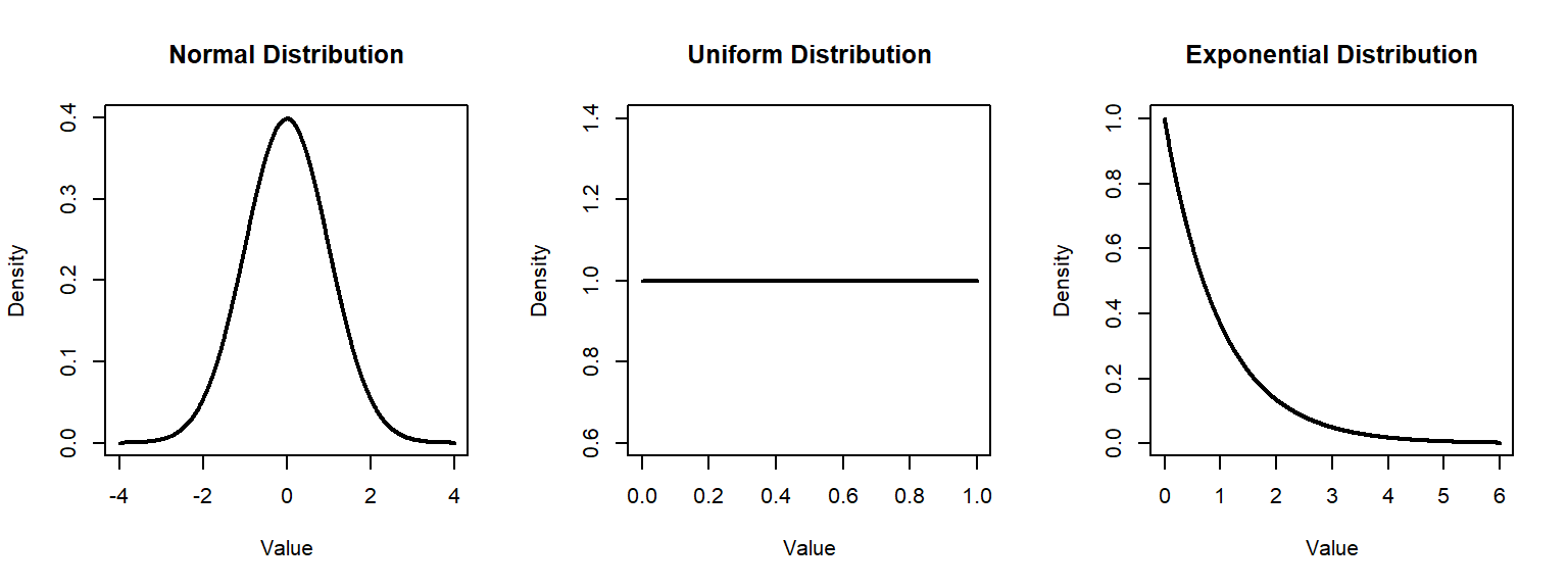
# Reset plotting layout
par(mfrow = c(1, 1))# Set up the x-axis values
x <- seq(-4, 4, length = 1000)
# Compute the density of the standard normal distribution
y <- dnorm(x, mean = 0, sd = 1)
# Plot the standard normal distribution
plot(x, y, type = "l", lwd = 2, main = "Standard Normal Distribution",
xlab = "Value", ylab = "Density")
# Shade the area above x = 2.5
x_shade <- seq(0.5, 1.5, length = 1000)
y_shade <- dnorm(x_shade, mean = 0, sd = 1)
polygon(c(0.5, x_shade, 1.5), c(0, y_shade, 0), col = "darkgoldenrod3", border = NA)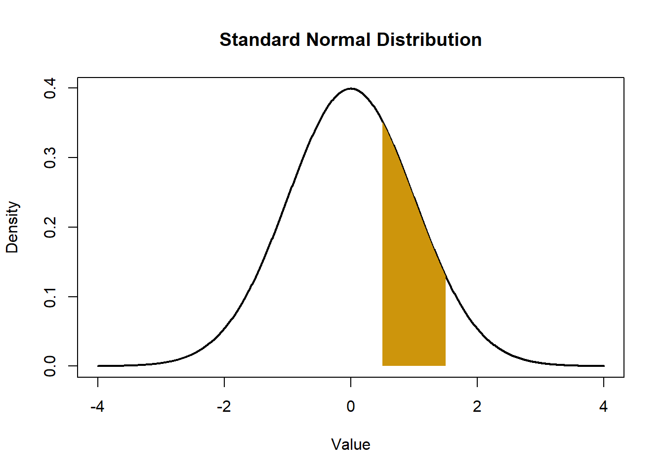
For the normal distribution,
\[f(x) = \frac{1}{\sqrt{2\pi \sigma^2}} \textrm{exp}\Bigl\{-\frac{1}{2} \frac{(x - \mu)^2}{\sigma^2}\Bigr\}\]
where \(\mu\) is the mean and \(\sigma^2\) is the variance.
You do NOT need to know this formula for the exam.
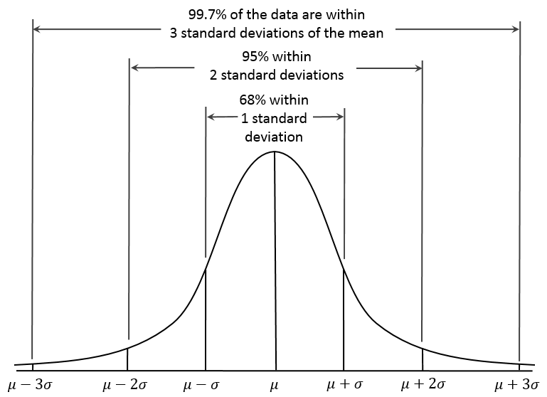
The normal distribution is a family of distributions of a specific form. There are an infinite amount of possible distributions, since \(\mu\) can be any real number and \(\sigma^2\) can be any positive number.
It would be very cumbersome to have to individually think about a \(N(0, 20)\) vs. \(N(2.5, 2)\) vs. \(N(694, 1549)\) vs. …. distribution, depending on the situation.
In practice, we could calculate a standard score or z-score that gives the number of standard deviations away from the mean an observation from a particular population is.
A z-score tells us how many population standard deviations an observation is away from the population mean.
They provide ways to compare results across many different measurement scales, since z-scores are unitless
\[z=\frac{x-\mu}{\sigma}\]
(note the use of population parameters \(\mu\) and \(\sigma\))
According to NHANES, the mean bone mineral density for a 65 year old white woman is 809 mg/cm\(^2\), with a standard deviation of 140 mg/cm\(^2\).
Suppose you are a 65 year old white woman whose bone density is 698 mg/cm\(^2\).
Should you be very concerned about osteoporosis?
Let’s calculate a z-score and find out!
Review discrete distributions
Poisson distribution and Alzheimer’s example
Continuous distributions, density functions
The normal (Gaussian) distribution
z-scores