qnorm(.975, mean = 0, sd = 1)[1] 1.959964BIOS 600 - Spring 2026
Exam scores will be ready next Tuesday, 2/24
Priority drop/add deadline looks like next Friday, 2/27?
HW 4 will be assigned later today and will be due next Thursday February 26 at 11:59pm.
Confidence intervals: what are they, and how do we interpret them?
qnorm() and pnorm(): useful functions in R and how to use them
Using a t-distribution vs. a z-distribution to create confidence intervals
P & G: Chapter 9
OpenIntro: No corresponding section.
A confidence interval gives a range of values that is intended to cover the parameter of interest to a certain degree of “confidence”
Confidence interval = point estimate \(\pm\) margin of error
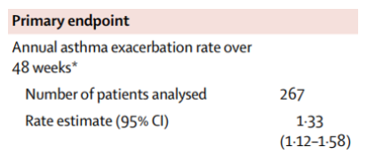
Researchers conducted a clinical trial of a drug intended for severe asthma patients. Their primary endpoint was evaluating whether the mean rate of asthma exacerbation over 48 weeks was different between placebo and treatment arms.
Above is the 95% confidence interval for the mean rate among the placebo patients.
How do you interpret this interval? (more on this very soon!)
For now, let’s assume that we know \(\sigma\), the population standard deviation (this rarely ever happens)
Recall from last lecture: Given a random variable \(X\) with mean \(\mu\) and standard deviation \(\sigma\), the CLT tells us that
\[Z = \frac{\bar X - \mu}{\sigma / \sqrt{n}}\]
where \(Z\) has a standard normal distribution if \(X\) is normal, and \(Z\) is approximately normal if \(X\) is not normal, but \(n\) is large enough.
\[0.95 = P(-1.96 \leq Z \leq 1.96)\]
\[(\bar X - 1.96 \frac{\sigma}{\sqrt n}, \bar X + 1.96 \frac{\sigma}{\sqrt n})\]
Generic form of confidence interval:
Point estimate \(\pm\) confidence multiplier \(\times\) standard error
Example: Suppose we specify \(\alpha = 0.05\), or a 5% significance level.
Since 95% of the area under the curve is contained within [-1.96, 1.96], we have 2.5% of the area to the right of 1.96 and 2.5% of the area to the left of -1.96.
In this way, we are interested in a \((1-\frac{\alpha}{2})100\)% or 95% CI.
Then, 1-\(\alpha/2 = 0.975\) and \((1-\frac{\alpha}{2})100\)% \(=97.5\)%.
We can find the 97.5 percentile (the 0.975 quantile) of the standard normal distribution in R with the qnorm() function:
qnorm(.975, mean = 0, sd = 1)[1] 1.959964qnorm doing in words?qnorm(p, mean, sd) is finding the quantile of the normal distribution distribution corresponding to \((p \times 100)\%\) of the area under the curve falling to the left of this value, assuming a normal distribution with mean and sd.What quantile of the normal distribution corresponds to 50% of the area under the curve?
qnorm(.5, mean = 0, sd = 1)[1] 0Answer: 0
alpha <- 0.05
qnorm(1-(alpha/2), mean = 0, sd = 1)
[1] 1.959964\[\textrm{Point estimate} \pm \underbrace{\textrm{confidence multiplier} \times \textrm{standard error}}_{\text{Margin of error}}\]
Examples:
Suppose we want a 10% significance level. Then \(\alpha\) = 0.1.
Then we have a \(1-\alpha/2 = 0.95\).
So, \(z^*\) is the 95\(^\text{th}\) quantile of the standard normal distribution (calculated using software packages)
qnorm(.95, mean = 0, sd = 1)[1] 1.644854The function pnorm(p, mean, sd) gives the probability underneath the curve, to the left of the value p.
Examples:
pnorm(1.96, mean = 0, sd = 1)[1] 0.9750021pnorm(3, mean = 0, sd = 1)[1] 0.9986501What will the following code return?
pnorm(0, mean = 0, sd = 1)?qnorm in your console to find out more info about these functions!\[(\bar X - 1.96 \frac{\sigma}{\sqrt n}, \bar X + 1.96 \frac{\sigma}{\sqrt n})\]
Suppose we select \(M\) different random samples from the population of size \(n\), and use them to calculate \(M\) different 95% CIs in the same way as above.
Approximately 95% of these intervals would cover the true \(\mu\) and 5% do not
Correct Interpretation: “If we were to repeat the study many times, constructing a 95% confidence interval each time in the same way, then about 95% of those intervals would contain the true population parameter.”
Another correct (more succinct) interpretation: We are 95% confident that the true mean lies within \((\bar X - 1.96 \frac{\sigma}{\sqrt n}, \bar X + 1.96 \frac{\sigma}{\sqrt n})\).
Note there is a big difference between “95% confident” and “95% probability”.
Pick a partner.
Click on the applet from 2 slides ago.
Each person should pick a number of confidence intervals to generate (over 50), then explain to their partner 1) how many of of their CIs generated contained the true parameter, and 2) how this relates to the idea of confidence.
How would you interpret this confidence interval?
A study estimates the mean systolic blood pressure of adults with diabetes as 132 mmHg, with a 95% confidence interval of [128, 136]
How would you interpret this confidence interval?
Is this interpretation correct?
“There is a 95% chance that the true mean SBP lies in the interval”
This is incorrect!
Important: we do not know whether any particular interval is in the 95% of them that cover the mean or the 5% that don’t
Since \(\mu\) is a parameter, it’s either in our confidence interval or not
\[(\bar X - z^* \frac{\sigma}{\sqrt n}, \bar X + z^* \frac{\sigma}{\sqrt n})\]
Remember, this is only ok to use when \(\sigma\) is known, and either:
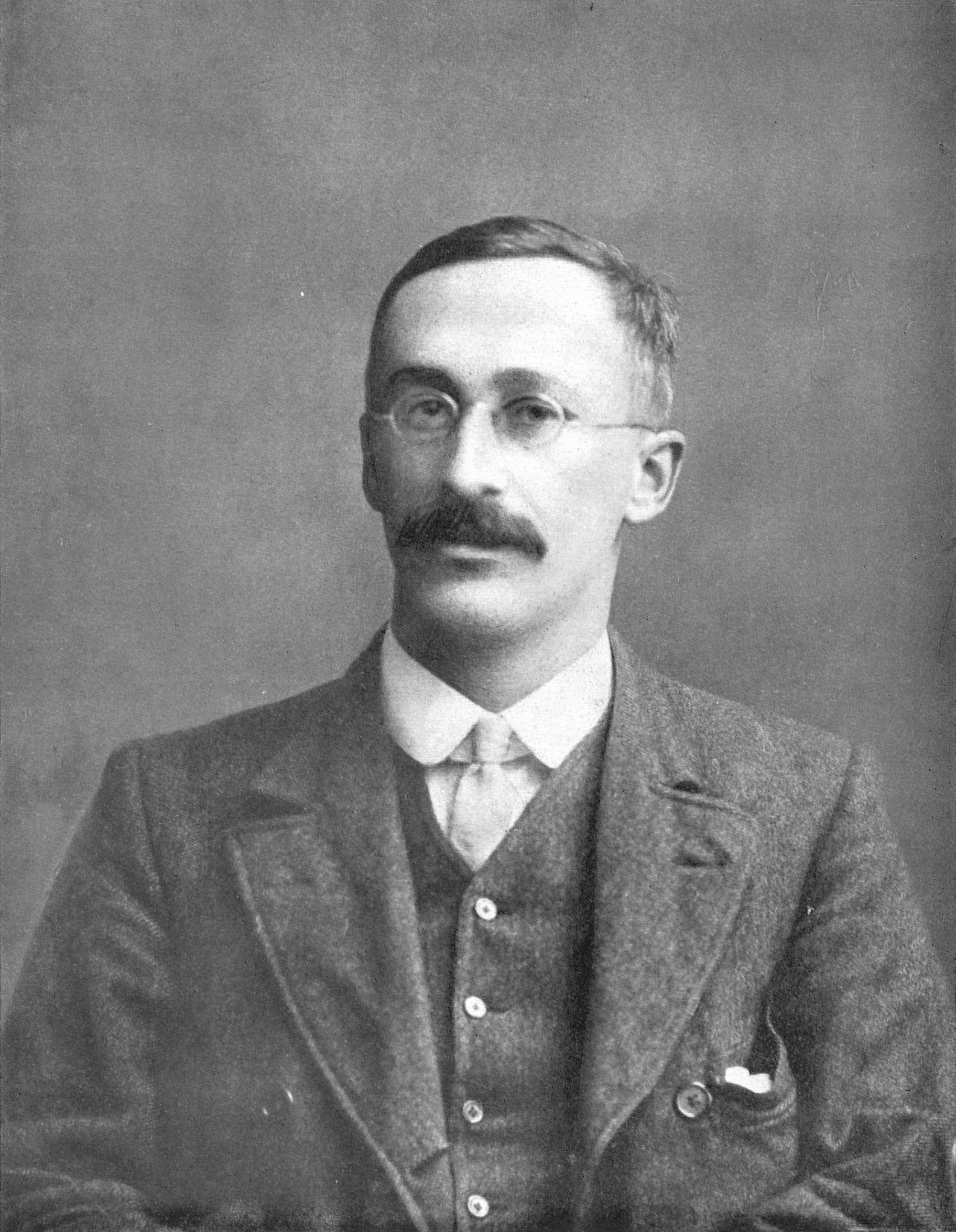
As a Guiness brewery employee, William Sealy Gossett published a paper on the \(t\) distribution, which became known as Student’s \(t\) (the brewery didn’t allow him to use his own name)
A. Student. The probable error of a mean (1908)
Gosset used his new distribution to determine how large a sample should be for testing beer
The \(t\) distribution is appropriate for constructing a confidence interval for the mean when \(\sigma\) is unknown
# Set up the x-axis values
x <- seq(-4, 4, length = 1000)

# Compute the densities for the t-distributions
y_t1 <- dt(x, df = 1)
y_t3 <- dt(x, df = 3)
y_t10 <- dt(x, df = 10)
y_t30 <- dt(x, df = 30)

# Compute the density for the standard normal distribution
y_norm <- dnorm(x, mean = 0, sd = 1)

# Plot the density for t-distribution with 1 degree of freedom
plot(x, y_t1, type = "l", col = "red", lwd = 2, ylim = c(0, 0.4),
     main = "Comparison of t-Distributions",
     xlab = "x value", ylab = "Density")

# Add the density for t-distribution with 3 degrees of freedom
lines(x, y_t3, col = "blue", lwd = 2)

# Add the density for t-distribution with 10 degrees of freedom
lines(x, y_t10, col = "green", lwd = 2)

# Add the density for t-distribution with 30 degrees of freedom
lines(x, y_t30, col = "yellow", lwd = 2)

# Add the density for the standard normal distribution
lines(x, y_norm, col = "black", lwd = 2, lty = 2)

# Add a legend
legend("topright", legend = c("t df=1", "t df=3", "t df=10", "t df=30", "Normal (0,1)"),
       col = c("red", "blue", "green", "yellow", "black"), lwd = 2, lty = c(1, 1, 1, 1, 2))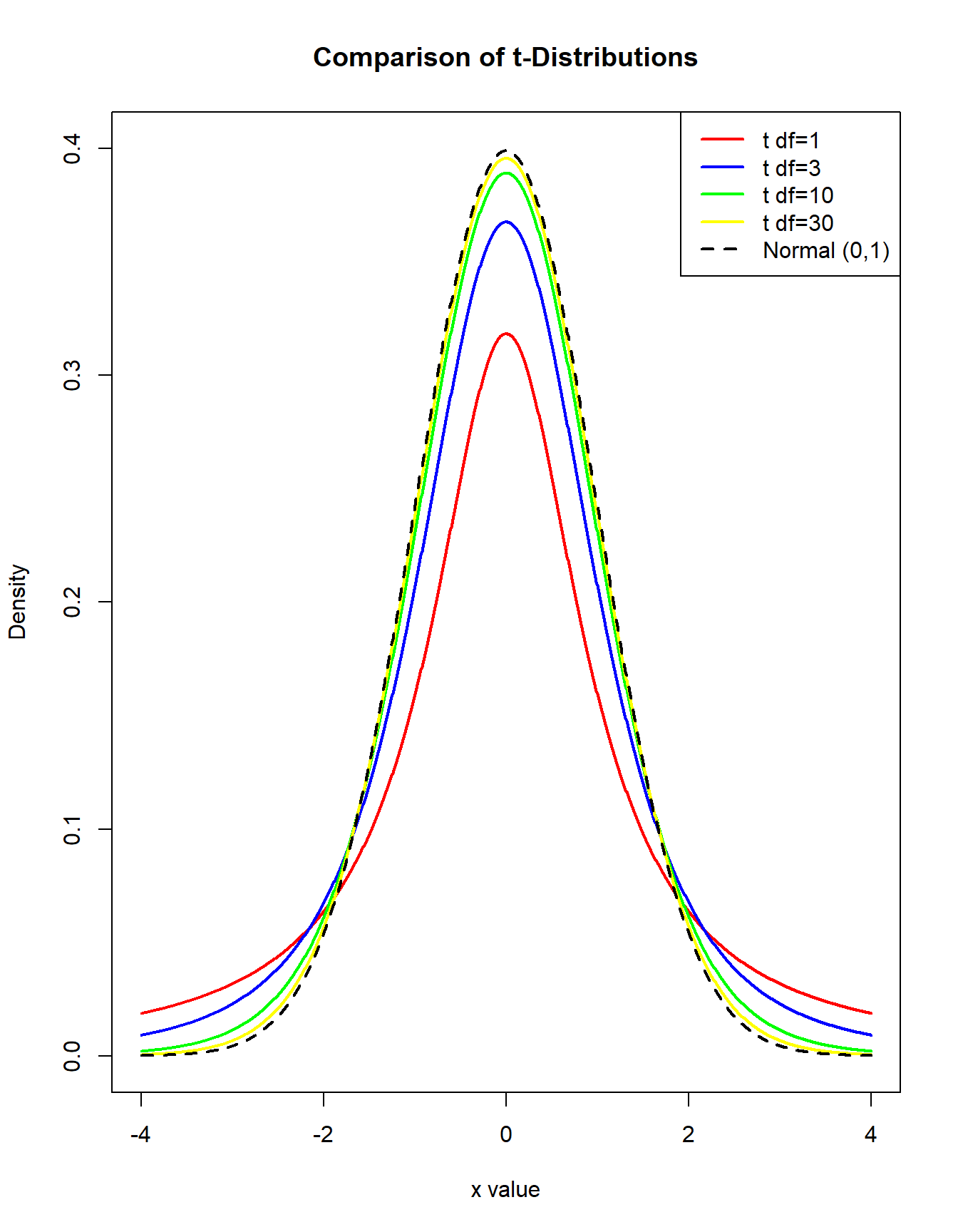
The \(t\) distribution looks like the normal distribution except it has thicker tails, leading to wider CIs
This is due to the uncertainty involved in estimating \(\sigma\) by using \(s\)
As the sample size increases, \(s\) is a better and better estimate of \(\sigma\), and so the \(t\) distribution looks more and more like the normal distribution
# Set up the x-axis values
x <- seq(-4, 4, length = 1000)

# Compute the densities for the t-distributions
y_t1 <- dt(x, df = 1)
y_t3 <- dt(x, df = 3)
y_t10 <- dt(x, df = 10)
y_t30 <- dt(x, df = 30)

# Compute the density for the standard normal distribution
y_norm <- dnorm(x, mean = 0, sd = 1)

# Plot the density for t-distribution with 1 degree of freedom
plot(x, y_t1, type = "l", col = "red", lwd = 2, ylim = c(0, 0.4),
     main = "Comparison of t-Distributions",
     xlab = "x value", ylab = "Density")

# Add the density for t-distribution with 3 degrees of freedom
lines(x, y_t3, col = "blue", lwd = 2)

# Add the density for t-distribution with 10 degrees of freedom
lines(x, y_t10, col = "green", lwd = 2)

# Add the density for t-distribution with 30 degrees of freedom
lines(x, y_t30, col = "yellow", lwd = 2)

# Add the density for the standard normal distribution
lines(x, y_norm, col = "black", lwd = 2, lty = 2)

# Add a legend
legend("topright", legend = c("t df=1", "t df=3", "t df=10", "t df=30", "Normal (0,1)"),
       col = c("red", "blue", "green", "yellow", "black"), lwd = 2, lty = c(1, 1, 1, 1, 2))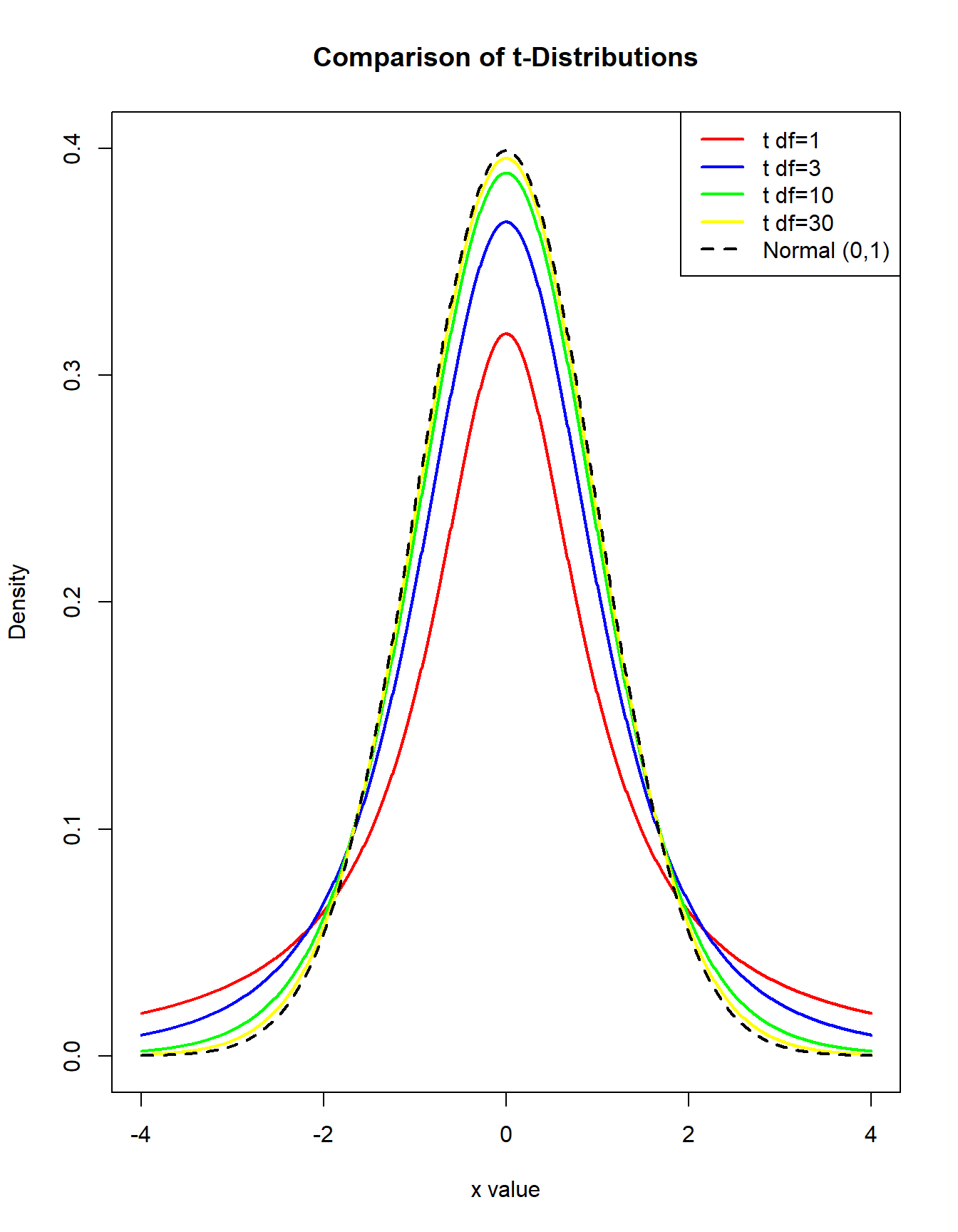
\[t = \frac{\bar X - \mu}{s/ \sqrt{n}}\]
has a \(t\) distribution with \(n-1\) degrees of freedom (\(df\)), which we denote by \(t_{n-1}\) (we lose one \(df\) by estimating the sample mean using \(\bar X\)).
The \(t\) distribution only has one parameter (\(df\))
How does this compare to the standard normal distribution?
\[(\bar X - t^*_{n-1; 1-\alpha/2} \frac{s}{\sqrt n}, \bar X + t^*_{n-1; 1-\alpha/2} \frac{s}{\sqrt n})\]
-In practice, if \(\sigma\) is unknown, we use the t-distribution no matter the sample size.
The symmetric two-sided confidence intervals we have dealt with so far give the shortest intervals with the desired coverage probability (for symmetric distributions)
Occasionally, we may only want an upper limit or a lower limit for the population mean, for instance in a non-inferiority clinical trial for a generic drug (we don’t expect the generic drug to work better, but we do expect it to be “not worse”)
We won’t focus on these in this class.
Confidence intervals: what are they, and how do we interpret them?
qnorm() and pnorm()
Using a t-distribution vs. a z-distribution to create confidence intervals